I N T R 0 D U C T 10 N

This chapter describes what you can infer about a population from a sample of observations drawn from that population. It focuses on inferences about population means and percents.' Examples of population means include the average annual per capita purchases by a population of customers, and average waiting time for customers trying to contact an airline reservation system. An example of a population percent is the percent of the United States workforce that is unemployed.

The key concept of statistical inference is that although a sample provides useful information about a population mean or percent, that information is imperfect. We are left with some uncertainty about its true value. Statistical inference provides ways of estimating the true value and of quantifying our uncertainty about that estimate.

Samples are taken when it is impossible, impractical, or too expensive to obtain complete data on a relevant population. For example, you ask a sample of people drawn from a target population how much each intends to spend on a product, and from their responses you make an inference about actual sales per capita for the whole target population. As another example, you take a sample of telephone calls coming into an airline reservation system, measure the amount of time (if any) each call is kept waiting, and from this make an inference about the average waiting time for all calls.

This chapter gives you a conceptual overview of issues in sampling and inference. Some of the basic ideas are subtle. The best way to test your understanding of these ideas is to work through the examples and the exercises. When you get a numerical result, ask yourself what that result means.
 
 

SAMPLING ERROR

A sample may fail to tell you the exact value of a population mean or percent 3 due to sampling error. Sampling error arises from the fact that the sample mean may differ from its counterpart in the population due to the "luck of the draw." It is one of several sources of error in making inferences about a population from a sample.

 Inferences from a Sample

Even if a sample is "representative" of the population from which it is drawn, it provides only imperfect information about that population, owing in part to sampling error. As an illustration, suppose you ask 100 potential customers how much they will spend on a proposed new product next year. The first says $10, the second $92, the third "nothing," and so on. You add up the 100 responses, divide by 100, and obtain $32.51 as your sample average. At this point, you want to make an inference from these responses about how much will be spent by the average potential customer in your entire market (the target population) next year. You could make the following inferences:

a) "My best estimate of average sales per potential customer is $32.51."

b) "Average sales per potential customer will be between $27.37 and $37.65 with 95% confidence."

c) "Average sales per potential customer will be greater than the breakeven amount of $27 at a 21/2% level of significance."

An inference like (a) is called statistical estimation, (b) is a confidence interval, and (c) is a test of (statistical) significance.

Estimation and Confidence Intervals

Statistical estimation is a relatively straightforward procedure: when the distribution of values in the population is fairly symmetric and there are no extreme outliers, the sample mean (m) serves as a good estimate of the population mean. In the sales per customer example, $32.51 serves as a good estimate of the population mean.

Confidence intervals, on the other hand, are somewhat more subtle. Confidence in how close a sample estimate is to the true population mean depends on the sample size (n), and on the dispersion of 5 the sample observations, as measured by the sample standard deviation (s). Everything else being equal, your uncertainty about the value of a population mean will decrease as the sample size increases and the dispersion in the sample values decreases. To illustrate, in the example above, you would feel more confident that the population mean is close to $32.51 if your sample mean of $32.51 came from a sample of 400 respondents, instead of only 100. Similarly, you would feel more confident that the population mean is close to the sample mean if each of your 100 respondents expected to spend between $32 and $33 on the product next year, and less confident if their responses ranged from "nothing" to $500.

The level of confidence about the value of a population mean can be expressed in terms of a confidence distribution. In making inferences about a population mean, the mean of the confidence distribution is equal to the sample mean m, and its standard deviation (called the standard error) is equal to the sample standard deviation s divided by the square root of the sample size, n:

standard error = s/(n)^1/2_

The standard error decreases as the dispersion in the sample decreases and as the sample size increases.

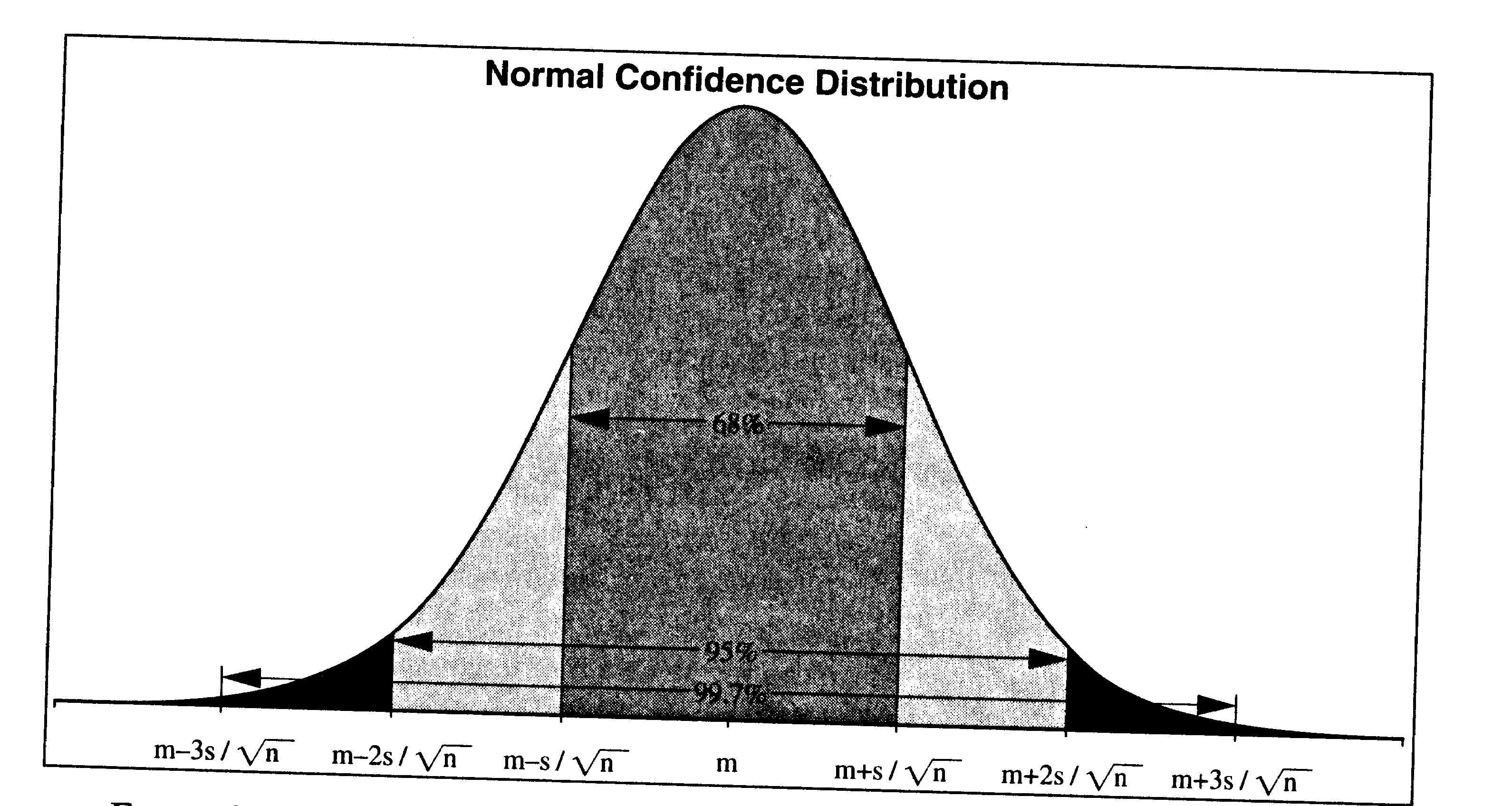
The shape of a confidence distribution is essentially normal or bell-shaped, regardless of the shape of the distribution of values within the population itself. As is the case for any normal distribution, a value within one standard deviation above or below the mean occurs with 68% confidence; a value within two standard deviations above or below the mean has 95% confidence; and a value within three standard deviations has 99.7% confidence. Figure 2.1 portrays these relationships for a confidence distribution.

From the confidence distribution, you can construct a confidence interval for the population mean. A confidence interval states both a range within which the true value of the population mean may lie, as well as a level of confidence that the population mean does, in fact, lie within that interval. Confidence intervals of different lengths, and correspondingly different levels of confidence, can be constructed from a given sample. In general, we would prefer confidence intervals to be narrow rather than wide, since narrow intervals imply greater certainty about the population mean, and we would like the confidence level to be as high as possible. Unfortunately, for a sample that has already been taken, these preferences constitute a tradeoff: the narrower the confidence interval, the lower the confidence that the true value of the population mean lies within the interval. Conversely, the higher you want your confidence to be that the population mean lies within a given interval, the wider the interval must be. The only way you can achieVE both objectives-to have a narrow interval with high confidence-is to take z large sample.

From the confidence distribution, you can construct a confidence interval for the population mean. A confidence interval is based entirely on three characteristics of a sample: the sample size, n; the sample mean, m; and the sample standard deviation, s. The population size is irrelevant. A confidence interval based on a sample with given values of n, m, and s will be the same, whether the sample in question is drawn from a population of 1,000 or a population of 1,000,000. It is a very common error for people to believe that an adequate sample should be some fixed percentage of the population, say 10%. Quite the contrary. It is the absolute size of the sample that determines accuracy.

The following example illustrates how a confidence interval is constructed. A market researcher asks a sample of 100 potential customers how much they plan to spend on a product next year. The mean of this sample turns out to be $32.51 and the standard deviation is 25.7. The best estimate of what the average potential customer will spend is, therefore, $32.51. The standard error is 25.7/(100)^1/2 = 25.7/10 = 2.57.
 Thus, with 68% confidence, 7 we can say that the average potential customer will spend between $32.51 - $2.57 and $32.51 + $2.57 (or between $29.94 and $35.08).

Similarly, with 95% confidence, average expenditure will be between $27.37 and $37.65, and with 99.7% confidence, it will be between $24.80 and $40.22.

Statistical Significance

A third type of inference you can make from a sample is a test of significance. Rather than estimating a point at which, or an interval within which, the population mean lies, you can indicate if the population mean is likely to fall above or below a critical value of interest, called c. For example, you may want to know whether average sales per capita is likely to exceed a breakeven level of $27. If the sample mean is $32.51 and thus lies above the critical value of $27, how likely is it that the population mean is on the same side of the critical value?

To answer this question, you can first construct a confidence interval and then determine whether the interval overlaps the critical value. If it does not, the sample outcome is said to be statistically significant. If it does overlap the critical value, the sample outcome is said to be not significant. These tests have a corresponding level of significance, and the two should be reported together. A sample result is statistically significant at a level of 21/2% when a critical value falls outside a 95% confidence interval, and therefore lies in a region in which we have only 21/2% confidence 8 that the population mean lies. Similarly, a test is statistically significant at a level of 0.15% when a critical value falls outside a 99.7% confidence interval.9

The case of launching a new product serves to illustrate tests and levels of significance. Suppose n = 100, m = 32.51, and s = 25.7. Then, as we saw before, a 95% confidence interval extends from 27.37 to 37-65, and does not cover the critical value of c = 27. Therefore, relative to 27, the sample outcome of 32.51 is statistically significant at the 21/2% level.

The t-statistic.

 Rather than determining statistical significance by constructing a confidence interval, the following shortcut procedure produces the same results. If c represents the critical value, compute the statistic

t = (m -c)/standard error= (m-c)1(s(n)^1/2 )

Then if t > 2 or t < -2, the sample outcome is significant at the 21/2% level. (Try the computation on the two examples above, and convince yourself that it yields the same results.) If t > 3 or t < -3, the sample outcome is significant at the 0.15% level.

Significance vs. Importance.
 
It is very important to realize that a result can be statistically significant but unimportant, or vice versa. Because it is extremely unlikely that the population mean or percent will be precisely equal to the critical value, a sufficiently large sample usually shows statistical significance, whereas smaller samples may not. For this reason, a statistically significant outcome may not be economically better than an outcome that is not statistically significant. For example, suppose a manager is trying to decide which of two new products, A or B, to introduce. Breakeven sales per capita are $27 for both A and B. The manager obtains a sample of 10,000 potential customers for product A, but only 100 for product B. The sample results are in Table 2.1.
For product A, a 95% confidence interval extends from 27.1 to 27.5, a result that is statistically significant relative to c = 27 at the 21/2% level. For product B, a 95% confidence interval extends from 26 to 66, and hence the result is not significant at the 21/2% level. If the manager must now decide which product to introduce, and can acquire no more data, what should she do?
 
 

	Product a	product b
n	10,000	100
m	27.3	46.0
s	10	100

Product A has higher prospects of breaking even, but not much potential for large profit. Product B has lower prospects of breaking even (more downside risk) but much more upside potential. Unless the manager were very risk-averse, she should prefer B to A.

 Sample Size

Taking a sample to obtain information about a population mean requires a decision about the sample size. How large a sample should you take? Since sampling is usually expensive, and the cost of sampling often increases with sample size, there is a tradeoff between more precision at higher cost and less precision at lower cost. To determine the appropriate sample size, you can first specify the length of a confidence interval and an associated confidence level that you would consider satisfactory, and then compute a sample size that will deliver such a confidence level and interval.

Suppose, for example, you want to say with 95% confidence that average annual expenditure for a target population is within an interval of length L. That is, if the sample mean turns out to be $32.51, you would like the sample size to be such that with 95% confidence you would know the population mean is between 32.51-0.5L and 32.51 + O.R. How large a sample must you take to achieve this level of precision? If we knew the sample standard deviation, s, the answer would be simple. You would like the interval from m - 2s sqr(n)

to m + 2s sqr(n) to have length L. That means that 4s /sqr(n)=L, or sqr(n) = 4s / L, or n = 16s^2 / L^2 . If s = 25.7 and L = 2, then the required sample size would be n = 2,642. (By similar logic, the sample size for a 68% confidence interval is n = 4S^2/L^2, and for a 99.7% interval is n = 36s^ 2 / L^ 2.)

A sample of this size might be prohibitively expensive. If you were willing to double the length of the interval L from 2 to 4, you could reduce the size of the sample by a factor of four, from 2,642 to 661. That is because the length of the interval depends on 1 sqr(n) : if you quadruple n, you halve the length; if you reduce n by a factor of 4, you double the length. In general, the process of choosing a sample size is an iterative one, in which you compare the tradeoffs between precision and cost.

The analysis above assumes that you know the value of the sample standard deviations before the sample is even drawn. Unfortunately, s is a statistic whose value is computed after the sample is drawn. The only thing you can do to escape this logical trap is to guess'O the value of s, and hope that your results are not too sensitive to a substantial

Suppose, as before, a sample of 100 potential customers reveals how much each will spend on your product next year. In the past several years, average expenditure per customer has ranged from $10 to $15, and no product or competitive changes are likely to support a jump to the $27 - $38 range. For this reason, you must conclude that the 95% confidence interval extending from roughly $27 to $38 overstates the probability that demand per customer will fall in that range. You can only conclude that the luck of the draw led to a sample mean of $32-51 that, in this case, was too high.

If, on the other hand, you have no additional information to suggest that this sample result is substantially more or less likely than other possible results, then you can interpret the confidence distribution derived from the sample as a probability distribution, and you can treat a significance level as the probability that the population mean falls above or below a critical value.

 Population Percents

As indicated previously, almost everything that we have said regarding inferences for population means applies to population percents. Although it is natural to think in terms of percents (the percent of voters who will vote for candidate X; the percent of people who will buy our product, etc.), it is important for computational purposes to express percents in fractional form, e.g., 20% = 0.20. To emphasize this, we will use the language of fractions and not percents in this section.

When we are dealing with fractions, individual values can be coded as Os and Is. A person who will vote for candidate X will be coded 1; a person voting for a different candidate will be coded 0, etc. The mean of this dummy variable is then the fraction of Is. Suppose we take a sample of n observations, and that a fractionf of those observations are 1s. Then the sample fractionf is the sample mean. Accordingly:

*The sample fraction f is an estimate of the population fraction.

*A confidence distribution for the population fraction is normal with mean f and standard error s / sqr(n) .

*The 68%, 95%, and 99.7% confidence intervals are defined exactly as before,  as are t values.  While the value of s can be computed for a dummy variable in exactly the same way as for any other variable, there is a shortcut formula available. For a dummy variable S

unless n is quite small (10 or less), the term n /(n-1) is close enough to 1 so that it can be safely ignored. Thus, to a very reasonable approximation,

Example. A sample of 100 voters was asked for which of two candidates, X or Y, they would vote. Fifty-two said they would vote for X. Then f = 0.52, S =,/-O.52 - (1- 0.52) = 0.4996, and the standard error is 0.4996/ sqr(100) = 0.04996. A 95% confidence interval would extend from 0.52 - 2*0.04996 = 0.4201 to 0.52 + 2*0.04996 = 0.6199. The sample outcome is not significant at the 2'h% level relative to a critical value of c = 0.50. (Had the sample size been 10,000, with 5,200 in favor of X, the sample outcome would have been statistically significant, as you should verify.)
 

Figure 2.2  shows how the standard deviation s for a dummy variable depends on the sample fraction f. If you are quite sure, before you take a sample, that the sample fraction will not be less than 0.2 nor greater than 0.8, you can be equally sure that s will be between 0.4 and 0.5.

This is very helpful in sample-size problems. To illustrate, suppose you are conducting a national poll to determine the percent of voters who will vote for the Republican candidate in the next presidential election. Suppose that you want to state with 95% confidence that your results are within an interval of L= 5 percentage points. We can be quite sure thatf will be between 0.2 and 0.8, and hence that s will be between 0.4 and 0.5. Let's assume the worst case-that s = 0.5. Then our sample size n should be such that

In fact, many national polls involve around 1,600 respondents, and are commonly reported as having a margin of error of 2 1/2% (half the length of the confidence interval); the confidence level of 95% is implicit.