One of the simplest rules by which a time series can be generated is the constant-average rule, which specifies that each value of the series is the sum of a constant, M, plus a disturbance; for the tth observation,

Neither M nor the values of et are directly observable, but inferences about them can be made by analyzing the data.

Simulating the Series. What does a constant-average series look like? We can artificially simulate such a series by specifying a value for M, a probability distribution for et and then drawing sample disturbances from this distribution. Suppose M = 10, T = 20, and et has a normal distribution with mean 0, standard deviation 2.5. Values of et should be such that each value is independent of prior values; in the long run, the average value should be 0, 68% of the values should be between -2.5 and + 2.5, 95% between -5 and + 5, 99.7% between -7.5 and + 7.5, the histogram should look appropriately bell-shaped,
and the cumugram should be appropriately S-shaped. Of course, in any sample, the actual values of et will fail to conform exactly to these criteria because of sampling error.

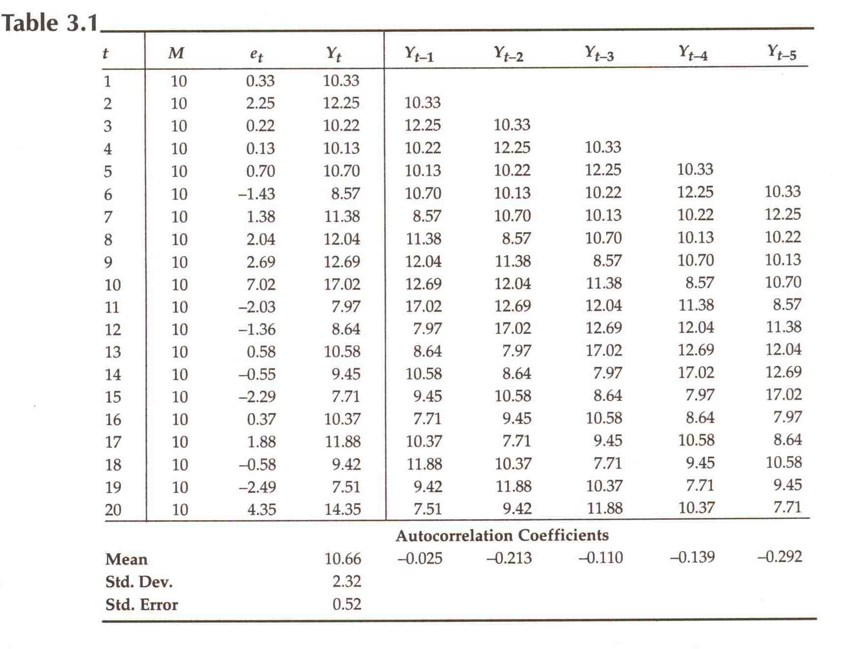
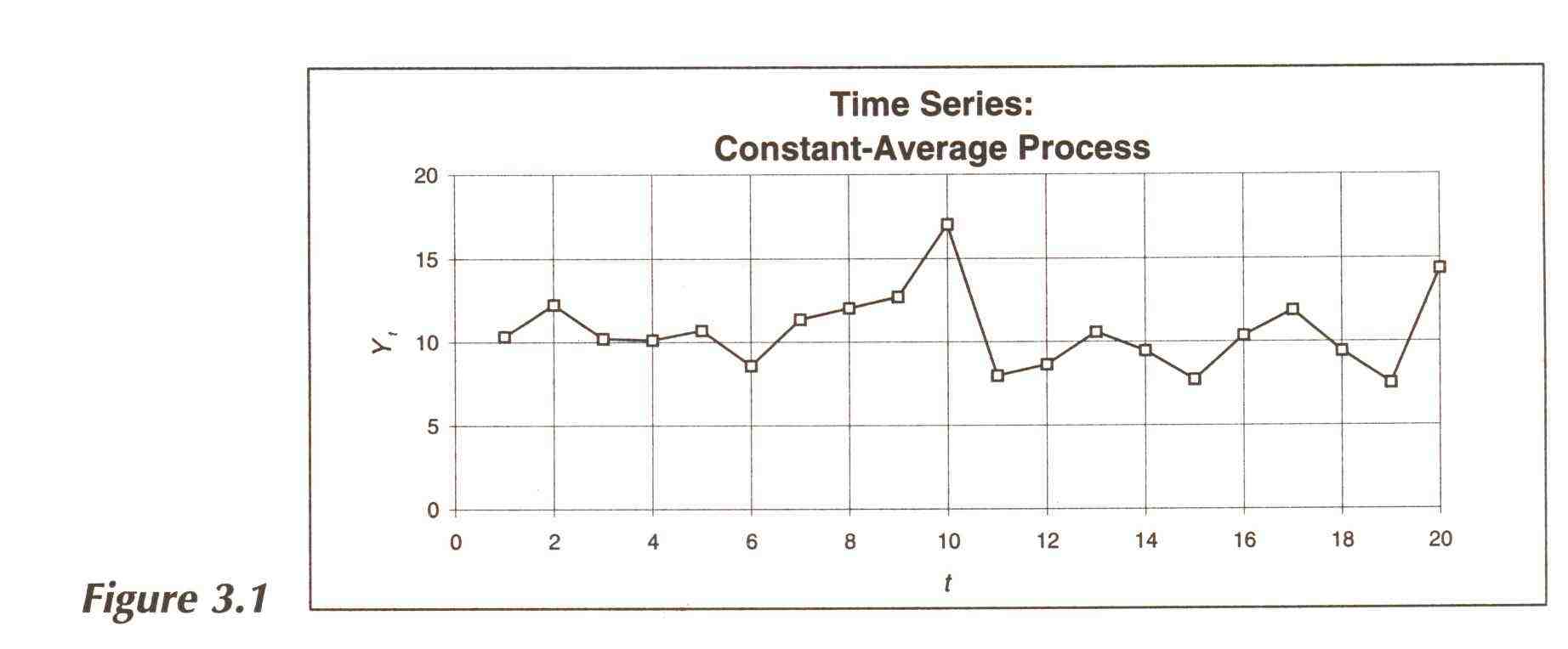
The first four columns of Table 3.1 shows values of the variable Yt generated in this way. Figure 3.1 shows values of Yt plotted as a time series.
 
 

Identifying the Rule. Now let's switch gears. Suppose we were presented with the 20 observations on Yt given in Table 3.1. If we knew what those observations represented, we might be able to identify the rule governing the data-generating process. For now we will simply ask how, by examining the data, could we check a hypothesis that those observations came from a constant-average process?

If that hypothesis were true, each observation would differ from M by an amount that does not depend on the value of the previous observation. Therefore, a scatter diagram of each observation plotted against its predecessor should show no correlation (except for sampling error). In column 5 of Table 3.1 we show Yt-1, the values of Yt lagged by one period.' Figure 3.2 is a scatter diagram, showing values of Yt-1 on the horizontal axis and values of Yt on the vertical. There is no discernible correlation. The coefficient of correlation between Y, and Yt-1 (the first-order autocorrelation coefficient), based on the 19 observations for which both variables have values, is -0.025; it is printed at the bottom of the fifth column in Table 3.1. We have not introduced the specific technique for computing the confidence distribution of a correlation coefficient, but it can be shown that when the population correlation coefficient is 0 and the sample size is 19, a 68% confidence interval will cover sample correlation coefficients between -0.24 and +0.24, and a 95% interval will cover -0.45 to + 0.45; thus the observed sample correlation coefficient of -0.025 is by no means inconsistent with the hypothesis that in a sufficiently large sample, Yt and Yt-1 would be uncorrelated.

We could now go on to create new variables consisting of two-period lags Yt-2, three-period lags Yt-3, etc., and for each of these compute the appropriate-order sample autocorrelation coefficient: a second-order coefficient based on the correlation between Yt and Yt-2, a third-order coefficient, etc. These coefficients are computed up to five-period lags, and are shown at the bottoms of their appropriate columns in Table 3.1. As we would expect, they are sufficiently close to 0 to be consistent with a hypothesis that process autocorrelation coefficients of all orders are 0. This is the key to identifying a time series as one generated by a constant-average rule: for such a series, sample autocorrelation coefficients of all orders will differ from 0 only because of sampling error.

Forecasting. Having identified the rule that governed the generation of the data, we can now try to make a forecast. If we knew that M = 10, and that the disturbances were normally distributed with mean 0, standard deviation S = 2.5, a "point" forecast for Y21 would be 10, and a probabilistic forecast would be between 7.5 and 12.5 with probability 0.68, between 5.0 and 15.0 with probability 0.95, and between 2.5 and 17.5 with probability 0.997. Unfortunately, we don't know the value of M, the standard deviation of the disturbances, or even that the disturbances are normally distributed. But the data provide estimates of M and S: the sample mean m = 10.66 is not very far from the process mean M = 10; and the sample standard deviation s = 2.32 is not very far from the process standard deviation S = 2.5. If the disturbances were normally distributed, then the values of yt in the sample of 20 observations should be approximately normally distributed; that this is so can be verified by plotting a cumugram of the actual values of yt and of a normal distribution with mean of 10.66, standard deviation of 2.32. Figure 3.3 shows such a plot; the fit is quite good.5
 
 

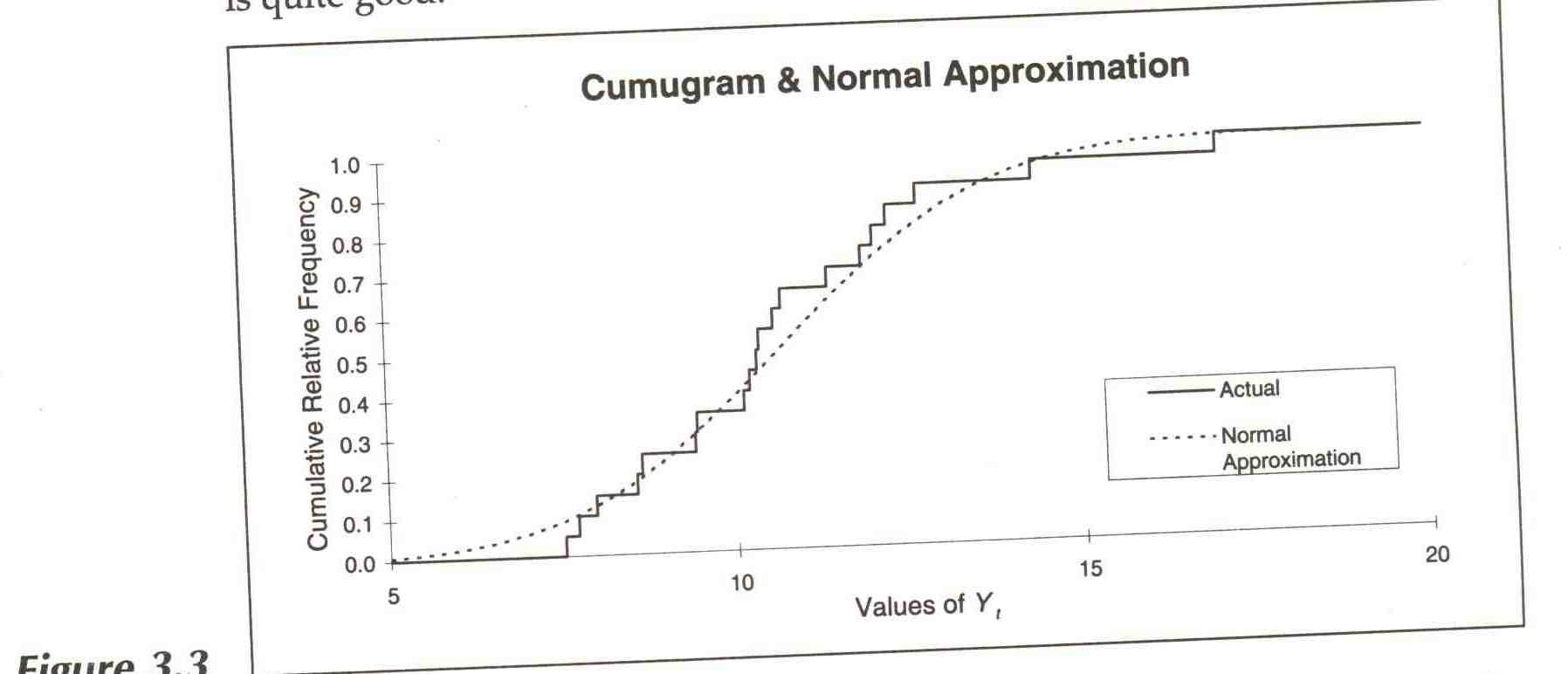
We can now either use the cumugram of actual values to make probabilistic forecasts or, more simply, use the normal approximation. Using the latter, we would get approximate probability intervals as follows: the value of y2l would be between 8.34 and 12.98 with probability 0.68; between 6.02 and 15.30 with probability 0.95; and between 3.70 and 17.62 with probability 0.997. These intervals are close to, but not exactly the same as, the ones we computed assuming we knew the values of M and S and the rule that governed the data-generating process for sure. In general, intervals computed in this way from sample data will be too narrow, on the average, because we have made four simplifying assumptions:

1. We are using the sample mean m instead of the process mean M.

2. We are using the sample standard deviations instead of the process standard deviation S.

3. We are assuming the disturbances are normally distributed, an assumption supported by, but not proved by, Figure 3.3.

4. We are assuming that the rule that governed the data-generating process was a constant-average rule, which is supported by, but not proved by, the autocorrelation analysis.

More sophisticated methods can make adjustments to take into account the first two simplifying assumptions, but only judgment can adjust for the third and fourth. For our purposes, just understanding that the intervals are somewhat too narrow is sufficient.

Suppose we want to forecast Y221 the value of y two periods ahead. If we knew the value of y2l, the value of y one period ahead, we could recompute m and s based on all 21 observations, and compute a point forecast and probabilistic forecasts based on these new statistics. But if we have only 20 observations in hand, and are looking two periods ahead, all we can do is use the values of m and s that are based on 20 observations: the forecasts for y22 and subsequent values of y are precisely the same as that for y2l.

There are thus two important characteristics of constant-average rules: both point forecasts and probabilistic forecasts of future values, no matter how far into the future, are all precisely the same; and all existing observations are equally important in determining forecasts of future values. The value of y, is as important in forecasting the value of y2l as is the value of y2o. As we shall see, these characteristics of constant-average rules do not apply to the next rule that we shall consider.

The Random-Walk Rule

A time-series observation generated by a random-walk rule is equal to its immediate predecessor plus a random disturbance:

yt = yt-1 + et

If the first observation is yo, then

yl=yo+el

Identifying the Rule Given the 21 observations y0 through Y20 shown in Table 3.2, can we see whether a hypothesis that the observations were generated by a random-walk rule is consistent with the data? An immediate consequence of the rule

yt = yt-1 + et

is that

yt - yt-1 = e,
The difference between each observation and its immediate predecessor (often called the first difference) is just a random disturbance. Thus, first differences behave as if they were generated by a constant-mean rule with M = 0.

We already know how to analyze data generated by a constant-mean rule: we look at lags of one, two, and more periods, and compute sample first-order, second-order, and higher-order autocorrelation coefficients. Here the lags are not on the values of the series, but on their first differences. If the autocorrelations on these first differences can be shown to be equal to 0 except for sampling error, then the first differences are consistent with a hypothesis that they were generated by a constant-mean rule, and therefore the values of Yt are consistent with a hypothesis that they were generated by a random-walk rule.

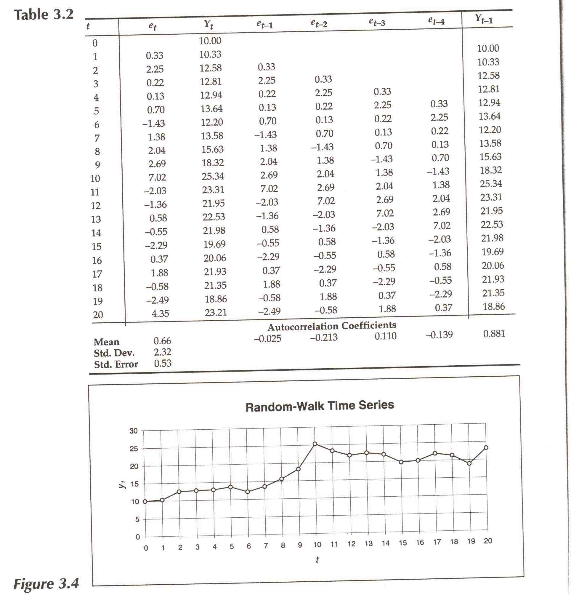
In columns 4-7 of Table 3.2 we show lagged first differences. (Column 2 shows values of the first difference itself.) At the bottom of columns 4-7 are the autocorrelation coefficients for the first differences. just as was true in the analysis of the constant-average process, sample autocorrelation coefficients ought to be between --0.24 and + 0.24 with confidence 68% if the process had zero autocorrelation; all the coefficients are within that interval.

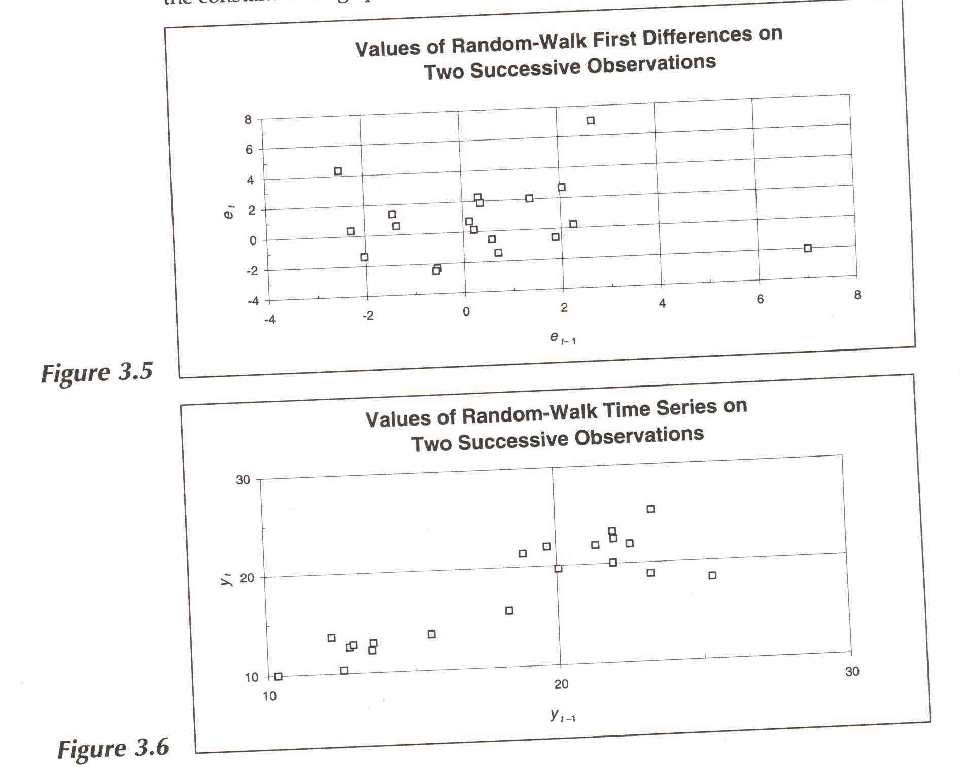
In Figure 3.5 we plot first differences lagged one period against "this period's'' first differences. There is no discernible correlation in the scatter diagram. Notice, however, that if we plot the lagged values of Yt given in column 8 of Table 3.2, against current values of the series itself Yt as in Figure 3.6, there is considerable correlation. (The correlation coefficient for oneperiod lags is 0.881.) Contrast this with the corresponding scatter diagram for the constant-average process.

Because the mean of e2l = 0, the best point forecast for Y21 is just the preceding value, Y20: the history of the process prior to the 20th observation is irrelevant to forecasts of the future. The same is true for point forecasts for Y22 and subsequent y's the best forecast is the last observed value.

Turning to probabilistic forecasts, y2l differs from Y20 by the disturbance e2l' All the disturbances have been assumed to be independently and identically distributed. We can infer their distribution from a histogram or cumugram of their values (they are just the values of the first differences themselves) or, if we assume the disturbances are normally distributed with mean 0, we can estimate the standard deviation of the distribution by computing the sample standard deviation of the disturbances. For the data in Table 3.2, the standard deviation is 2.32. Thus, since Y20 = 23.21, a probabilistic forecast for Y21 is between 20.89 and 25.53 with probability 68%, between 18.57 and 27.85 with probability 95%, etc. As was true in the case of the constant-mean process, these intervals are somewhat too narrow, for all the same reasons.

What is the distribution of the sum of two iid disturbances? It can be shown that if each disturbance has a normal distribution, the sum also has a normal distribution. Furthermore, the mean of the sum is the sum of the means, or 0, and the standard deviation of the sum is s sqr( 2 , where s is an estimate of the standard deviation of the distribution of any one disturbances Thus a forecast for y22 will lie in the interval Y20 ± s sqr(2) with probability 68%, etc. For the data in Table 3.2, Y22 will be between 19.96 and 26.46 with probability 68%, between 10.20 and 29.72 with probability 95%, etc.

These results can be generalized. If the last observed value in a random walk is yT, then a probabilistic forecast of yT+n will have mean yT+n and standard deviation s sqr(n) : the further