Multiplicative Symmetry: A Second Look

In our discussion of histograms earlier in this chapter we showed that some variables have multiplicatively svmmetric distributions. We stated, without any justification, that the logarithmic transformation of some variables has a distribution that exhibits ordinary symmetry. The reason for this is not hard to Understand if you recall one key fact about logarithms; the logarithm of the product of two or more numbers is the sum of their logarithms.

Thus, for example, log(a*b*c) = log(a) + log(b) + log(c) .

This is true whether you are using so-called natural logarithms (logarithms to the base e, where e - 2.71828, approximately), or logarithms to the base 10. You should convince yourself, using a spreadsheet or a calculator, that

log(2+3*4) = log(2) + log(3) - log(4)

for both natural logarithms and logarithms to the base 10.

Distributions that are multiplicatively symmetric often arise when value of each observation is the product of a number of small random effects. The logarithm of such a value will then be the sum of a number of small random effects and the distribution of such a set of values is lNely to be symmetric. Thus, logarithms convert or transform multiplicative effects into additive effects.

Multiplicative Seasonals and Constant Growth Rates

If you turn backto Figure 1.7, the graph of retail sales over time, you will notice that the amplitude of the swings behvesm the December peak and the JanuaryFebruary trough seems to get larger over time. One possible explanation is that the seasonal effect is multiplicative. Supposse, for example, that every December tends to be 20% above normal and every January 15% below normal, then  the difference between December and January will be larger for high levels of sales, and smaller for low levels. Because the level of sales has been increasing over time, the differences will therefore get larger over time. If the seasonal effect of each months, in fact, a constant multiple of some Normal level of sales, then a graph showing a time series of the logarithm of sales will depict seasonal effects that add to or subtract from normal the same constant amount for each month: on the logarithmic scale, the seasonal effects will not change with tile level of the series. Figure 1.14 shows such a graph, it seems to confirm the multitalicative-seasorial hypothesis.

A constant . growth rate means that successive values in a time series are constant multiples of preceding values. For instance, if a variable increases by 5% per year, each year's value will be 1.05 times the preceding year's. 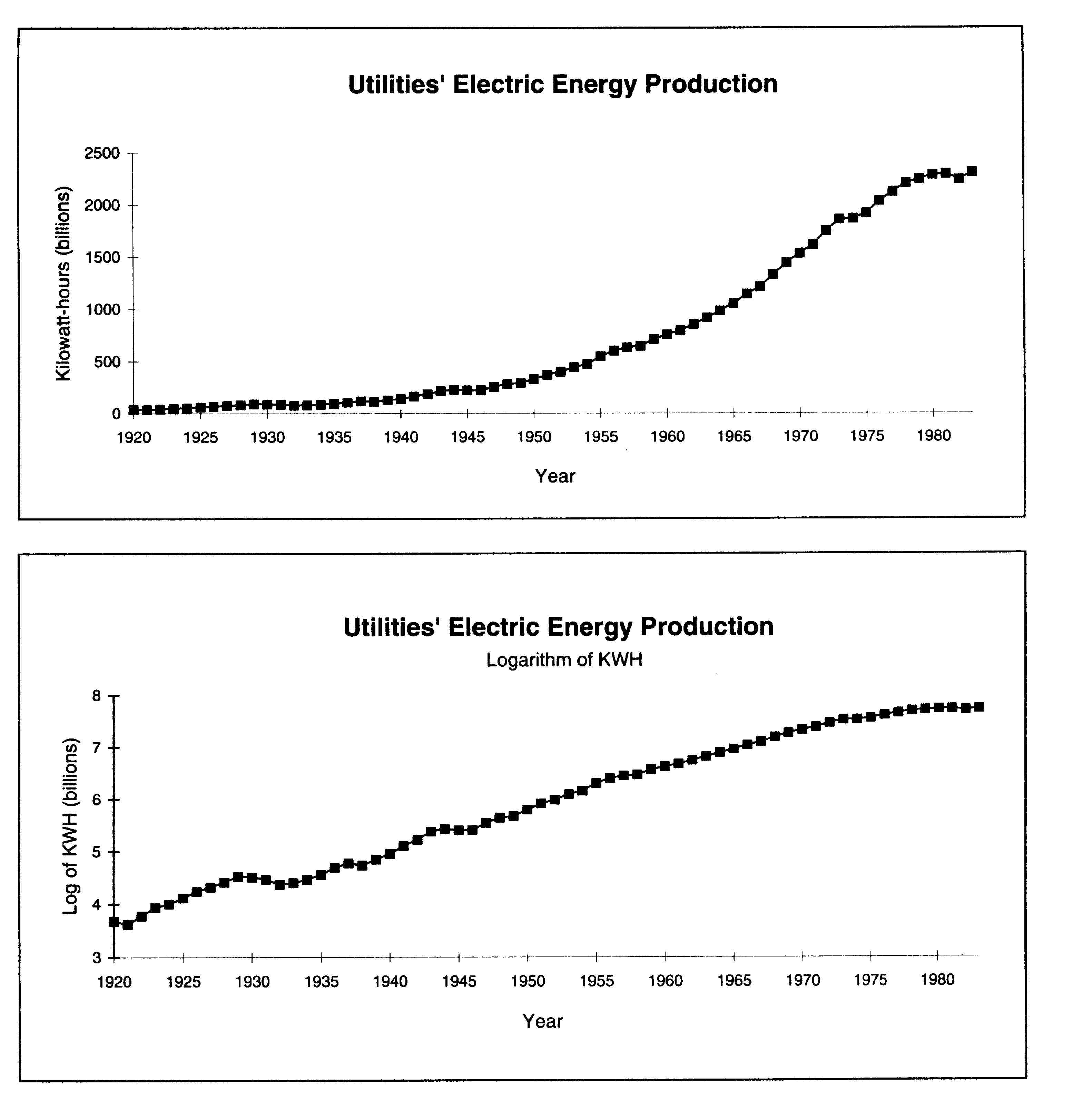If this is so, the logarithm of the values in the time series will have values that are constant increments above preceding values, and therefore a graph of the logarithmic series will have a shape close to a straight line. The U.S. population, the consumer price index, gross national product, and electric power generation all exhibit patterns of multiplicative growth over sufficiently long periods of time. The values increase at an increasing rate, often described as exponential growth. Figure 1.15, a graph of electric energy production in the United States from 1920 to 1983, exhibits this kind of exponential growth, at least through the mid-1970s. Figure 1.16, a graph of the logarithm of the series, is more nearly linear. Notice that by "linearizing" the series we can more easily detect the effects of the 1930s depression, the end of World War 11, and the OPEC oil crisis of the 1970s on energy production.

Multiplicative Effects in Cross-Sectional Data

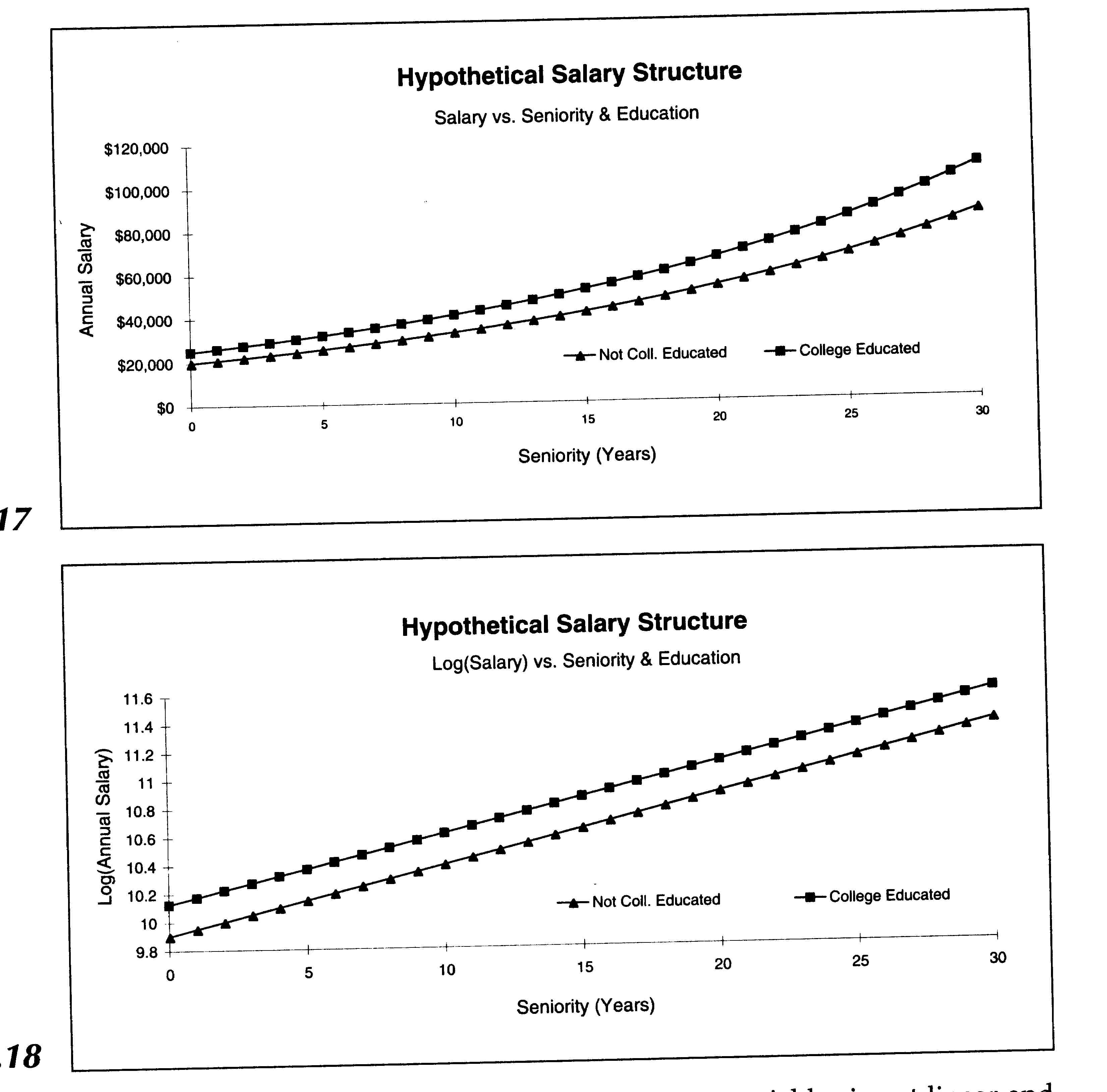
Even in cross-sectional data, the values of a variable may depend on the values of other variables in a multiplicative way. A companys salary structure may reward seniority and education, among other things. Suppose that in a given year starting salary for a person without a college education is $20,000, that college-educated employees earn 25% more than employees with comparable seniority, and that each year of seniority confers 5% more salary. Figure 1.17 shows what salaries would be if there were no additional factors affecting salary. Figure 1.18 shows the effects of seniority and education on log(salary). For a given level of seniority, education adds the same amount to log(salary), no matter what the level of seniority; we say that the effect of education on log(salary) is multiplicative. When we look at the effect of seniority on log(salary) for either level of education, we observe that it is linear, and this implies that the effect of seniority on salary is multiplicative.

In general, when the relationship between two variables is not linear and the dependent variable is measured on a ratio scale, it is a good idea to see whether effects can be more simply explained by looking at graphs of the logarithm of the dependent variable. A logarithmic transformation of a ratioscale dependent variable may:

* produce a symmetric, rather than a skewed, distribution of the dependent variable.

* produce a linear and additive relationship between the independent variables and the transformed dependent variable, if the effects on the natural dependent variable were multiplicative.

In performing transformations on our data, such as a log transform, we trade off complexity to get simplicity in the form of straight lines and additive effects.

Graphs with Logarithmic Scales

Ordinary graphs are plotted on an arithmetic scale, so that each increment on an axis represents equal distance (i.e., the distance from 1 to 2 is the same as the distance from 2 to 3). Sometimes graphs are plotted on a ratio or logarithmic (log) scale, in which equal distances represent equal percent changes (i.e., the distance from 1 to 2 is the same as the distance from 2 to 4).