LOGNORMDIST(x,my,sy) which calculates the cumulative distribution function,
where my = ln(mx) – ½sy2 and sy = ln[1+(sx/mx)2]. (Ayyub 1997)
Probabilistic Characteristics of M, c, I, fy, and
sThe probabilistic characteristics of s were calculated by statistical analyses on all four variables involved in s calculation as well as on s itself. After the initial set of random numbers was generated, histograms were created for M, c, I, and fy. This section describes the results for each of the four variables and then also for s.
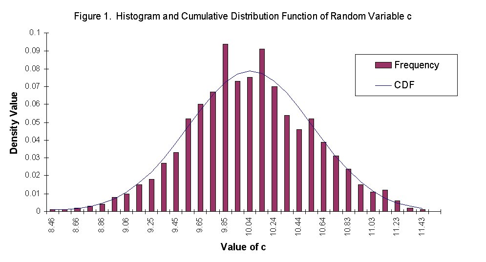
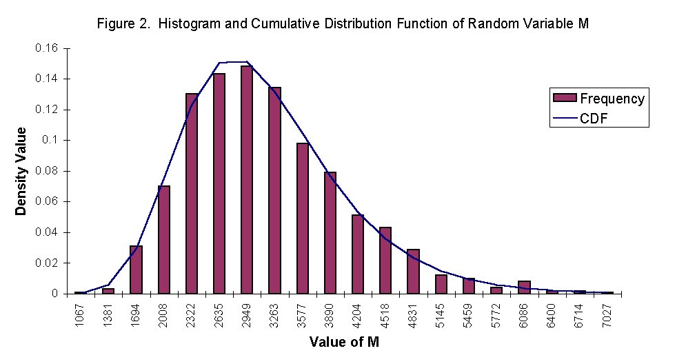
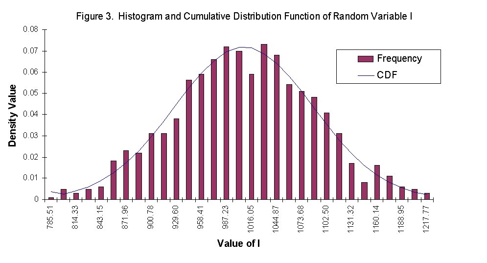
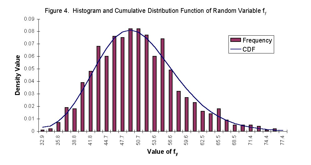
Histograms and Cumulative Distribution Functions for M, c, I, and fy
In order to illustrate the distribution types for each of the random values, plots of the cumulative distribution functions and the histograms were generated. We attempted to use the formula from Chapter 2 in Probability, Statistics, and Reliability for Engineers to establish the number of bins initially. The plots generated were not very clear and did not show the smooth relationship that the Histogram tool in Excel produced. Using the formula produced 11 bins and Excel determined 30 bins. The Excel tool bases the bin selection on the amount of dispersion in the data and subjectively creates the bin ranges.
The cumulative distribution functions were calculated using the following Excel equations. For the lognormally distributed variables M and fy:
LOGNORMDIST(x,my,sy) which calculates the cumulative distribution function,
where my = ln(mx) – ½sy2 and sy = ln[1+(sx/mx)2]. (Ayyub 1997)
For the normally distributed variables c and I:
NORMDIST(x,m,s,true) which calculates the cumulative distribution function,
 . (Ayyub 1997)
To view the generated plots of both the cumulative distribution functions and the histograms for c, M, I, and fy, click on the link below. In all cases, the randomly generated numbers fit very closely with the probabilities calculated for each distribution.
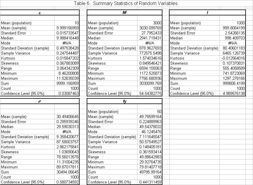
Statistical Analyses for M, c, I, and fy
Full statistical analyses were performed for the randomly generated variables M, c, I and fy and are displayed in Table 6. The statistics shown in Table 6 were generated using Microsoft Excel’s Descriptive Statistics tool. The means for each variable sample were calculated by the following formula:  . (Ayyub 1997) In all four cases, the sample mean is very close to the population mean given in the problem statement. The standard error for each was within 10% of the actual values. The standard deviation for each variable was calculated by the following:
  . (Ayyub 1997) The standard deviation for all four variables also fell within an acceptable range. Calculations for M yielded the highest standard deviation and standard error of the four variables, but they were still within reason. Sample variance was calculated as S2. The skewness was also measured for each of the variables. The formula used to calculate skew is as follows:
  . (Ayyub 1997) Other information recorded by Microsoft Excel’s Descriptive Statistics tool included kurtosis, maximum, minimum, sample count, and confidence level. As a result of the statistical analyses of M, c, I, and fy, no significant discrepancies exist in the random numbers generated for each. All numbers fall within a reasonable range of error and therefore are reasonable for calculating s.
Statistics of Random Variables (Table 6)
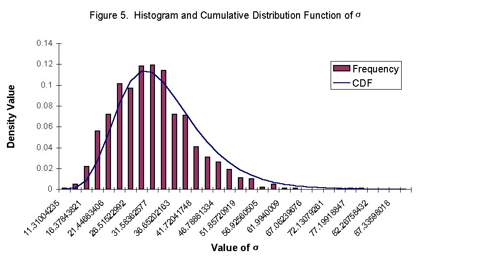
Discussion of Histogram, CDF, and Statistical Analysis for
sUsing the random variables generated for M, c, and I, the corresponding s values were calculated using the formula given in the problem statement:  . The resulting s values then were plotted as a histogram and the cumulative distribution function for each bin was calculated assuming that s followed a lognormal distribution. The probabilities calculated for s based on the CDF function discussed earlier were very close to the histogram bins when plotted together in Figure 5. The statistical analysis (see Table 6), performed in the same manner as described previously, also showed that the calculated s values fell within a reasonable range of error and, therefore, further analysis could be completed.
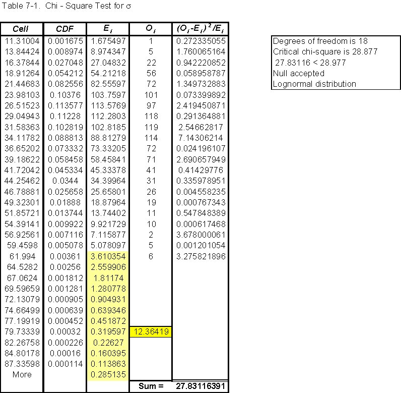
Chi-Square Test for Goodness of Fit for
sVisual inspection of the Sigma Histogram suggests a lognormal distribution of s. To determine if this assumption was correct, a chi-square test for goodness of fit was performed on s. The first step for the chi-square test was to formulate the hypotheses (indicated by the following):
Ho: sstress ~ LN(m,s)
HA: sstress ¹ LN(m,s)
Next, the appropriate model must be selected. Since this is the chi-square test, that’s the model used to test the hypotheses. Then, the test statistic must be identified. It is a random variable and is as follows:  . A level of significance must then be chosen. The level of significance chosen for this test was 5%. Next an estimate of the test statistic must be calculated. The estimate of the test statistic is computed with the procedure shown in Table 7-1 and the histogram in Figure 5. In order to determine the goodness of fit, a region of rejection must be defined. For degrees of freedom = 18 and a level of significance = 5%, the critical value of the test statistic obtained from table A-3 in Probability, Statistics, &Reliability for Engineers is 28.877. The region of rejection consists of all values of the test statistic greater than 28.877. Once the test statistic has been evaluated, the appropriate hypothesis must be selected. Because the computed value of the test statistic is less than the critical value, the null hypothesis is accepted and the lognormal distribution for s is appropriate.