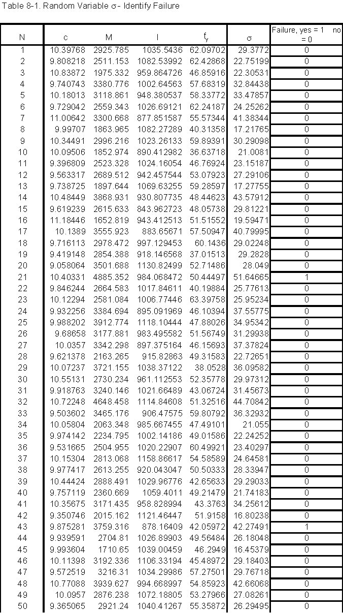
 . For each set of random variables, failure/non-failure was determined and a 1 was recorded in the Failure column of
 Yield Stress Exceedence Probability and Error Analysis
The yield stress exceedence probability provides the means to analyze the number of failures in comparison with the sample size. By determining this, the probability of steel beam failure can be better assessed because it directly correlates to the yield stress exceedence probability. The steps taken to compute the yield stress probability are explained below along with the results of that process.
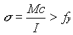
In order to begin calculating the yield stress exceedence probability, the number of failures must first be computed. As we know from the problem statement, failure occurs when . For each set of random variables, failure/non-failure was determined and a 1 was recorded in the Failure column of
Table 8-1 if failure occurred.
The total number of failures (Nf) for the sample was then computed. For the 1000 cycles included in this report, Nf = 72. Once the number of failures was calculated, the probability of failure (Pf) was computed using Nf and the sample size (N). The formula used to calculate Pf is as follows:
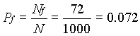 .
.
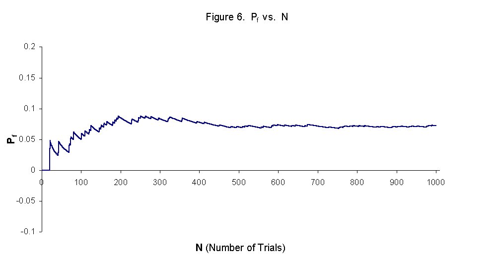
A graph showing the probability of failure versus the sample size is included as Figure 6. The graph indicates that the relationship between Pf and N varies greatly when N is small and gradually converges to the calculated Pf of 0.072 near 450 or 500 trials.
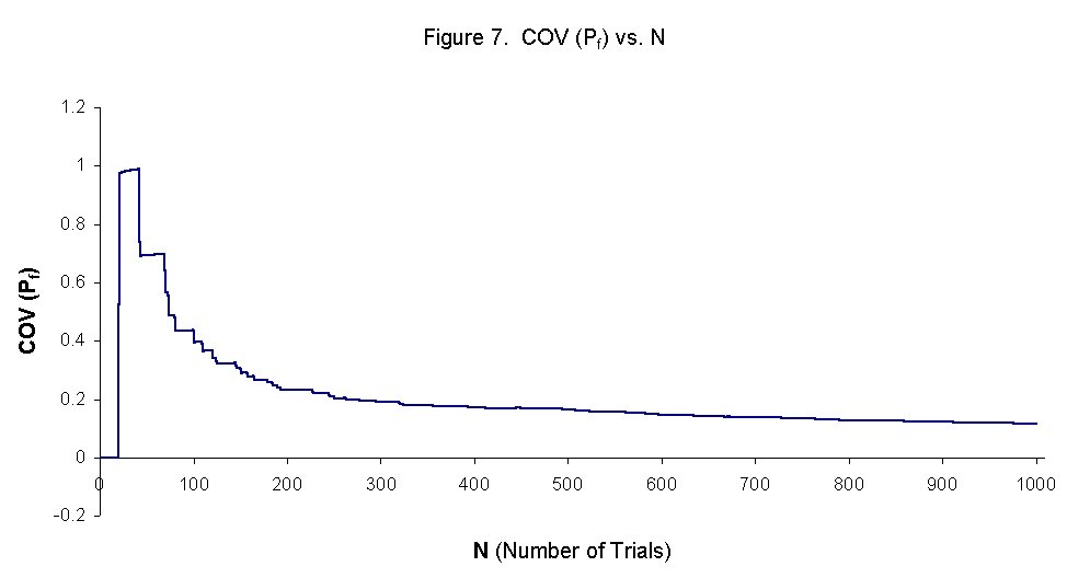
The coefficient of variation, COV, is used as a measure of error. It is an expression of the standard deviation in the form of a percent of the mean. To determine the COV, the variance of the probability was computed first by the following equation: 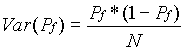 . For the computed values,
Var(Pf) = 0.000066816. The COV was then computed by the following equation: 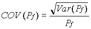 . For the computed values, COV(Pf) = 0.113529242 = 11.35%. The COV is graphed against the sample size, N, in Figure 7. The graph clearly shows that the COV converges as the sample size increases.