First, we shall enumerate the classical, widely-used procedure for calculation of the friction pressure drop. To do this, we formulate a practical situation: 80,000 barrels/day of wet oil, is to be pumped from a gathering station, through a pipeline 10" in diameter to a dehydration terminal 30km away. The operating liquid head at the terminal is equivalent to 3 bar(g) and therefore the wet crude must arrive at the tank with at least this pressure head. We wish to estimate the required discharge pressure of the export pump at the gathering station. Additional known data are as follows:
| Water cut | 28% |
| Dry oil viscosity | 30 cp |
| Dry oil density | 900 kg/m3 |
| Associated water density | 1020 kg/m3 |
| Pipe internal surface roughness | 0.03 mm |
The classical procedure for calculating the pressure drop, and therefore the required pump discharge pressure is as follows:
1) Calculate the effective liquid properties. The density is calculated as the weighted mean of those of the component oil and associated water. That is,
Effective density = (0.3 x 10²⁰) + (0.7 x 900) = 936 kg/m3
Effective viscosity is either calculated by Woelflin's correlation, or by the weighted arithmetic mean method as already discussed.
2) With the pipe diameter and the desired flow rate given, Reynold's number is calculated. With this, a decision is taken whether the friction factor should be calculated from Poisseuille's equation or from Colebrook-White's. Colebrook-White's equation would only be used if the procedure is being implemented in a computer program, otherwise, either one of the (simplified) explicit equations, or even published chart, is used to obtain the friction factor.
3) Having found the friction factor, pressure drop is computed by Darcy's equation. The pressure drop, plus the required discharge pressure (3 bar) is the minimum discharge pressure at the gathering station.
Not only with respect to emulsion viscosity calculation, but in some other respects, the above procedure is highly simplified and could lead to significant errors under certain conditions. We will look at the potential sources of significant errors in the procedure:
All the enumerated theories for calculating emulsion viscosity assume that the wet oil behaves as a homogeneous liquid in the pipe, and that our only problem is deriving the effective viscosity of that homogeneous liquid. In fact, this is not the case. At reduced flow rates, emulsification reduces. At sufficiently low flow rates, the oil and water actually separate out in the pipe, the oil flowing on top of the water. Clearly, assumption of a homogeneous liquid is unacceptable here.
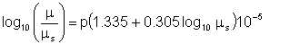
Both pressure and temperature affect liquid viscosity. The effect of pressure increases with the pressure - see fig. 3-1. The accepted equation for correcting liquid viscosity for pressure, when the viscosity at the standard condition is known, is as follows:
|
| Eqn 3/1 |
where μ = viscosity in Pa.s at pressure p, p being in kPa(g) and
μs = viscosity in Pa.s at 101.325 kPa.
The question arises: Since there is a pressure gradient along the line (that is, the pressure varies from inlet to outlet), at what pressure should the viscosity, or indeed, any other property of the fluid be calculated?
In their recommendation for gas flow, the California Natural Gas Association (CNGA) recommends that if p1 and p2 are the fluid pressures at pipe inlet and outlet respectively, fluid properties should be calculated for pressure p, given by:
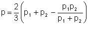
| Eqn 3/2 |
The logic of this is not clear, since for a uniform, horizontal pipeline, pressure drop is directly proportional to the distance from inlet, indicating that effective pressure for property evaluation should be a simple arithmetic average of the inlet and outlet. The CNGA suggestion gives a slightly higher effective pressure, and therefore higher pressure drop than would a simple average.
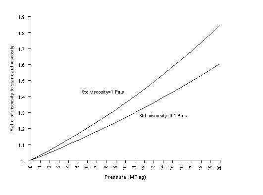
Fig. 3-1 Variation of liquid viscosity with pressure
In a study of the flow of two liquids and gas, Sobocinski and Huntington set a water-oil ratio of 0.66 with a total mass-liquid rate of 34,100 lb/hr/sq ft. This liquid rate was then made to flow with increasing gas rates. Table 1 is a summary of the types of flow and the formation of emulsions.
The pressure losses encountered by emulsified flow were found to be much greater than those under the same liquid and gas flow rate for non-emulsified flow. For example, it was found that for a total liquid rate of 35,300 lbm/hr-sq ft, a water-oil ratio of 4, and a gas rate of 13,000 lbm/hr-sq ft, the pressure gradient was 1.4 lbf/sq ft/ft. Under the same conditions of total liquid flow rate of 35,300 and a gas rate of 13,000, the pressure gradient was 0.28 lbf/sq ft/ft for water and air and 0.29 lbf/sq ft/ft for oil and air. As pointed out by Tek in his discussion of this work, the pressure drop for emulsified flow was five times that of flowing only air and water or air and oil.
| Air rates (Lbm/hr-sq ft) | Description |
| 2,000 | The oil flowed on top of the water at 150% of the linear velocity of the water. There was no disturbance between the air, oil and water boundaries. (Stratified flow) |
| 2,000-3,000 | Gentle ripples appeared on the oil surface but the surface between the oil and water remained smooth. |
| 3,000-4,000 | Linear velocity of oil increased to 227% of the water and deep ripples appeared on the oil surface with minor irregularities on the water- oil surface. |
| 4,600 | Waves appeared on the oil surface causing incipient emulsification. |
| 5,000-12,000 | Emulsification became very pronounced. It gradually encroached up the pipe walls, forming a continuous film around the entire inside periphery of the pipe. A greater portion of the emulsion remained on the bottom of the pipe. |
| 14,000 | The in-place ratio of the two liquids approached the flowing ratio, indicating that there was no slippage of the liquids. |
Charles, Govier and Hodgson carried out tests which showed that several flow regimes are possible, depending on velocity, density difference between the phases, volume ratio, and the interfacial tension. The phase distribution could vary from oil-continuous to water-continuous, from small contact area between the phases (slug flow or stratified flow) to large contact area (mist flow), and from apparently homogeneous distribution of the two phases (mist flow) to highly non-homogeneous (stratified flow).
The term "holdup", originally defined for 2-phase gas-liquid flow, was defined for water-oil flow as the ratio of the input oil-water ratio to the local or in-situ oil-water ratio. Some important conclusions from the tests are:
(a) Addition of water to an oil flow can reduce the pressure drop. For instance, pressure gradients at 0.3 fps superficial water velocity were approximately 10% of those for the oil alone. Of course, higher pressure drops can also be obtained by addition of water.
(b) Lower pressure drops are usually associated with oil flowing along the centre of the pipe (as bubbles, slugs, or core) at velocities which are higher than average, and surrounded by a sheath of water.
(c) Suspension of oil is difficult to achieve in systems with large density differences. In these cases the phases remain stratified, at least within the range of velocities presented.
(d) Phase stratification is likely to occur when
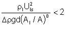
| Eqn 3/3 |
where ρl and Δρ are the lighter phase density and density difference between phases respectively, Uls is the light phase superficial velocity (based on the entire pipe cross-section), Al /A the ratio of the area occupied by the light phase to total cross-sectional area, d the pipe diameter, and g the gravitational acceleration. This is said to be valid where the light phase occupies more than 50% of the pipe cross-section.
Since the properties of liquids in a stratified flow cannot be assigned "mixture values", a different procedure is required for calculation of the pressure drop. Pressure drop in this situation correlates well in terms of Lockhart-Martinelli parameters. These parameters, first defined for gas-liquid flows, are:
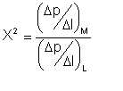
| Eqn 3/4 |

| Eqn 3/5 |
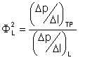
| Eqn 3/6 |
where the subscripts L and M denote the less and more viscous phase respectively, subscript TP represents two-phase conditions, and Δp/Δl is the pressure gradient. The single phase gradients are calculated as if the particular phase under consideration were flowing alone in the pipeline at a velocity equal to its actual, local superficial velocity. Lockhart and Martinelli proposed that there exists a unique relation between Φ and X. Work at Shell's research laboratory in Amsterdam (KSLA) showed that where both liquids have nearly identical densities and viscosities, the following relationships correlate ΦM and X:
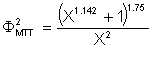
| Eqn 3/7 |

| Eqn 3/8 |
where ΦMTT2 = correlation for the case when both phases are turbulent, and
ΦMLL2 = correlation for the case when both phases are laminar.
Although this method is reliable, the need to first construct the applicable curve for the mixture at hand, before reading values from the graph limits its use for complex situations. This is especially so when dealing with pipeline networks.
Emulsification is promoted by low interfacial tension and high shear rate or velocity. It is possible only when the flow is turbulent, and provided that
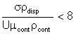
| Eqn 3/9 |
where σ is the interfacial tension, ρdisp and ρcont the dispersed and continuous phase density respectively, μcont the continuous phase viscosity, and U the bulk velocity. It points out that the continuous phase must usually be present at concentrations greater than 30%.