If we have an emulsion, with a certain droplet size distribution profile discharged from a pump into a pipeline at the pipe inlet, the droplet size distribution in the emulsion received at the pipe outlet would not be the same as what went in. The reason for this is that as the wet oil flows in the pipe, the pipe acts as a coalescer. The travelling time in the pipe amounts to a residence time during which tiny droplets fuse into larger droplets, and partial phase stratification takes place. The extent to which this occurs depends among other things on the flow turbulence, other devices in the line, and the length of the pipeline. Devices such as control valves exert considerable shear on the liquid, thus contributing to emulsification. The import of this is that emulsification index varies continuously along the pipe.
For this concept to be of use, it must be quantified. That is, we need to develop a relationship with which the emulsification profile can be predicted. We start by considering the phase separation principle derived from Stoke's law.
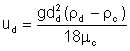
By Stoke's law, the velocity of migration of a dispersed phase droplet is given by
|
| Eqn 6/1 |
If hd is the average "escape" distance that a droplet must travel in the continuous phase to a region dominated by its own phase, then the time required for the escape of a dispersed phase droplet of diameter dd is (hd)/ud. That is,
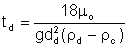
| Eqn 6/2 |
If the whole fluid is travelling in the pipe at an average velocity of U, then, during the time td, distance Ld travelled by the droplet along the pipe is (U x td). That is,
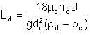
| Eqn 6/3 |
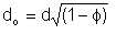
Conversely, the average diameter of water droplets that would have escaped to the water section over the length of the pipe is given by
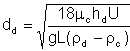
| Eqn 6/4 |
The process of coalescence of droplets is responsible for the "hold-up" in relation to the liquid-liquid 2-phase flow. Concentration of the dispersed phase in the bulk fluid varies along the pipe.
This author defines parameter hd as the droplet escape distance.
Consider the pipe transporting wet oil of water cut φw. If by some means complete separation of oil and water took place, then the water would occupy a proportion of the cross-sectional area of the pipe equal to φw, the oil occupying 1-φw.
We shall consider the situation whereby water is the dispersed phase, and oil the continuous phase. At the start of the journey of the wet oil in the pipe, the oil and water are well mixed up. As the journey progresses, the water droplets migrate to the bottom of the pipe. Let points oo and wo indicate the mid-point of the vertical depth of what would be the cross-section of the areas occupied by oil and water respectively. We can reasonably state the following:
If a water droplet of diameter dw at point oo succeeds in travelling to point wo before the whole fluid gets to the end of the pipe, then on the average, water droplets still in the "oil area" would generally be less than dw in diameter. Conversely, the average diameter of water droplets still remaining in the oil region at the end of the journey depends on the length of the pipe.
We can now define the droplet escape distance as the distance between the centres of the area portions of the cross-section of the pipe that would be occupied by the phases if the phases were completely separated in the pipe.
It can be shown that, on the average, hd equals half the pipe diameter, i.e.

| Eqn 6/5 |
>We will now illustrate application of these relationships with an example:
2000m3/d of oil with 20% water-cut is discharged from a centrifugal pump into a 6-inch diameter pipeline, 10km long. From the pump parameters, it is known that the average water droplet size at the pump discharge is 80μ. We wish to estimate the effective liquid viscosity at the pipeline outlet, assuming that is no coalescence or break-up of the dispersed phase droplets en route.
| Fluid data: | |
| Dry oil viscosity | = .05 Pa.s |
| Emulsion viscosity constant | = 3.5 |
| Oil density | = 900 kg/m3 |
| Associated water density | = 1020 kg/m3 |
| Interfacial tension | = .028 N/m |
| Pipeline data: | |
| Pipeline diameter | = 6 x .0254 = .1524 m |
| Pipe cross-sectional area | = π x .15242/4 = .01824 m2 |
| Average flow velocity | = 2000/(24 x 3600 x .01824) = 1.28 m/s |
| Droplet escape distance | = .5 x .1524 = .0762 m |
| Equation 6/4 gives ddisp | = [18 x .05 x .0762 x 1.28/(9.81 x 10000 x (1020 -900))]5 |
| = 86 x 10 -6 m or μ |
This means that water droplets 86* and larger would have separated out at the pipe bottom.
| Initial mean droplet size | = 80μ |
| For beta with assumed α=3 equation 2/23 gives β | 9 + (27/5) x 1.28 = 16 |
| Expected value of droplet size | = α/(α+β) = .16 |
Since this is equivalent to 80μ, maximum droplet size = 80/.16 = 500μ
The proportion of water that will have separated out is obtained by evaluating P(dp(x)>86) in equation 2/21. For the purpose of that integral, a = α-1 = 2, b = β-1 = 11. Thus we wish to evaluate
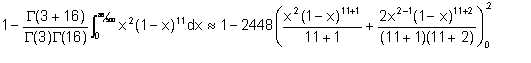
| Eqn 6/5a |
= 0.61
This indicates that 61% of the water will have separated out from the oil, indicating that 39% of the water still remains in the oil.
The 39% of the water that remains in the oil will have a maximum droplet size of 86μ. Assuming the same beta distribution parameters α and β, this translates to an average droplet size of .16 x 86 = 14μ. This corresponds to an emulsification index at the pipe outlet equation 2/29
Ei,out = 1 - .333log10(14) = 0.62
Now, if 39% of the original 20% water-cut in the wet oil remains in the oil, this indicates that the water-cut in the final emulsion phase is .39 x .20 = .078. Thus we have an emulsion with an emulsification index of 0.62 and a water-cut of 0.078. This emulsion will have viscosity equation 2/24
μe,out = 0.62 x (.05 x e3.5 x .078) + (1 - .62) x (.922 x .05 + .078 x .001)
= 0.058 Pa.s
In effect, what comes out of the pipeline is a 2-layer liquid - the bottom layer of water, and the top layer of emulsified oil having a viscosity of .058 Pa.s, from a water-cut of 7.8%.
Let us examine equation 6/4 again. Bearing in mind that the smaller the average droplet diameter that escapes, the less the emulsification, a low dd means a low Ei. It tells us that the process of demulsification is directly proportional to the square root of the distance travelled along the pipe, and inversely proportional to the square root of the flow velocity.
That is the emulsification index varies in proportion to the square root of flow velocity, and the inverse of the square root of the distance travelled.
This author proposes that stratified oil/water flow in a pipe be considered as flow in two pseudo-pipes each carrying one of the phases. Water flows at the bottom of the pipe. We can develop the model of an imaginary pipe such that the hydraulic behaviour of the water flowing in this pipe is equivalent to that of the water flowing in the bottom part of our real pipe. We can model a similar pseudo-pipe for the oil phase flowing on top of the water. The diameter and roughness of each pseudo-pipe can be expressed in terms of the water-cut, real pipe diameter and roughness.
If the total volume flow rate in the pipe is Q, and the pipe inside diameter is d, the bulk flow velocity is given by

| Eqn 6/6 |
If the water-cut is φ, then the cross-sectional area of the pipe occupied by water is

| Eqn 6/7 |
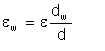
This must be the cross-sectional area of the water pseudo-pipe. The diameter of the water pseudo-pipe dw is thus given by

| Eqn 6/8 |
whence

| Eqn 6/9 |
The roughness of the pseudo-pipe is defined in terms of the real pipe roughness, diameter, and pseudo-pipe diameter as follows:

| Eqn 6/10 |
or
| Eqn 6/11 |
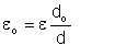
Similarly, we can state the dimensions for oil pseudo-pipe as follows:
| Eqn 6/12 |
and
| Eqn 6/13 |
Our next step is to calculate Fanning friction factors for each of our pseudo-pipes. For each pseudo-pipe, we calculate Reynolds number NRE. Depending on the value of NRE, we will calculate the pseudo-pipe friction factor from either Poisseuille's equation or Colebrook-White's. If the pseudo-pipe friction factors are fnw and fno respectively, the effective friction factor for the real pipe is
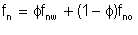
| Eqn 6/14 |
We can use this friction factor in Darcy's equation in the normal way.
We earlier (section 4.3) made reference to Sleicher's equation. In his study of concurrent flow of immiscible liquids in pipelines, Sleicher established that the droplet size of the dispersed phase, if initially very fine at high concentrations, increases as the distance downstream increases, owing to coalescence. If the droplets are initially large, they break up in regions of high shear (high turbulence). The maximum droplet size is given by
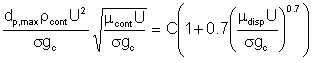
| Eqn 6/15 |
where
dp,max = maximum droplet diameter, ft
C = 43 (dt = 0.0417), or 38 (dt = 0.125), with
dt = dp,max/4 for high flow rates and dp,max/13 for low velocities, ft
gc = gravitational conversion factor, 4.18(10)8 (lb.mass)/(ft.)/(lb.force)hr2
U = superficial velocity, ft./hr.
σ = interfacial tension, lb.force/ft.
μ = viscosity, lb.mass/(ft.)(hr.)
If we take an average of C=40, rearrange and re-cast the equation in our chosen notation and adopt SI units, we obtain
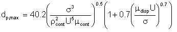
| Eqn 6/16 |
Wet crude oil flowing in a pipeline, with the following parameters:
| Water-cut = 20%, i.e. φ | = .2 |
| Interfacial tension σ | = .028 N/m |
| Dry oil density ρcont | = 900 kg/m3 |
| Associated water density ρdisp | = 1020 kg/m3 |
| Flow velocity | = 3 m/s |
| Dry oil viscosity | = .05 Pa.s |
| Associated water viscosity μdisp | = .001 Pa.s |
These data give a maximum water droplet size of 6.8 x 10⁻⁵ m or 68 micron. With the same data but a velocity of 1 m/s, the maximum water droplet size increases to 975 micron. At 0.5 m/s, the maximum water droplet size is 5490 micron.
The broken-up droplets (from the pump discharge) of the dispersed phase may start to coalesce into larger droplets, or further break up into smaller droplets, depending on the flow parameters. As we have seen with Sleicher's equation, the velocity of flow in the pipe determines the maximum droplet size that can stably exist in the pipeline: If the droplet diameters from the pump discharge are smaller than the maximum predicted by Sleicher's equation, coalescence of the droplets continues during flow. If the droplets at the pump discharge are larger than the maximum predicted by Sleicher, the droplets break up further. Whether or not the droplets coalesce or break up to the maximum predicted size would depend on the length of the pipeline: If the pipeline is sufficiently long, the droplets grow or break up in size until the maximum droplet size is as predicted by Sleicher's equation.
In example 6-1, if we recognise the effect of coalescence, then we must apply Sleicher's equation 6/16 to determine the maximum size to which the droplets tend to grow or break up:
dp,max = 456 x 10-6m = 456μ
Recalling that we started with a maximum droplet size of 500μ at the pipeline inlet, this indicates that there a slight breaking-up of the water droplets in the pipeline. This effect should be taken into consideration in a rigorous analysis. To do this, we need to know how the dispersed phase droplet sizes vary along the pipeline. Then, we would be able to estimate the point along the pipeline at which the droplet sizes stabilise (i.e., cannot coalesce or break up any further), if it does stabilise. The following discussion alludes to an approach that could lead to a useful relationship for such prediction.
Let us recall the Colebrook-White equation for calculating Fanning friction factor:
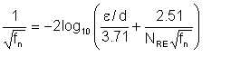
| Eqn 6/17 |
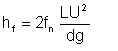
| Eqn 6/18 |
in which hf is the loss of head in friction. We pointed out earlier (section 1.6) that what we call friction pressure loss actually comprises two components. One component is due to the roughness of the pipe - pressure loss due to friction between the fluid and the internal wall of the pipe. The second component is due to friction within the fluid molecules. By inspection of Colebrook-White equation, we recognise these two components. The first term in braces accounts for the pipe roughness - it derives only from the surface roughness of the pipe in relation to the pipe diameter. The second term in braces derives from the dimensionless parameter Reynolds Number, and, implicitly, the overall friction factor itself. We note that Reynolds number derives only from the fluid properties and flow rate:
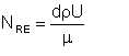
| Eqn 6/19 |
Thus, the second term in braces in the Colebrook-White equation represents the fluid friction loss due to internal friction within the fluid molecules. This author wishes to make the distinction between the overall flow friction, and its two components - pipe friction and fluid friction. We see that fluid friction is determined by:
For the case of a smooth pipe, we pointed out that the first term in braces becomes zero for the smooth pipe. The equation therefore reduces to:
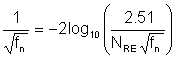
| Eqn 6/20 |
We know that for laminar flow, friction factor derives from Poiseuille's equation:

| Eqn 6/21 |
Laminar flow is characterised by isolation of the bulk of the flowing fluid from the pipe surface by the boundary layer, such that whatever may be the roughness of the pipe is of no consequence to friction loss. Both equations 6/20 and 6/21 imply the non-effect of the pipe surface roughness. Yet, they do not yield the same friction factor fn. To be sure, if we adopt equation 6/21 for turbulent flow (for which it is not intended), the friction factor we obtain by it is always less than what we obtain with equation 6/20. Figure 6-1 illustrates this point. This observation has significance for emulsification.
Figure 3 : Fanning friction factor for smooth pipe
Could the difference between friction factors obtained by equations 6/20 and 6/21 for the same Reynolds Number have something to do with the emulsification process?.
What becomes of the friction pressure loss? How is it expended? If the fluid loses energy due to friction, the energy must appear in some other form or forms. What readily comes to mind is conversion of such energy to heat (manifested as a slight, possibly imperceptible rise in the fluid temperature), sound (which is usually audible, especially at high flow rates), and vibration (which can be felt by touching the pipe). But, part of the energy is also expended in break-up of the liquid into smaller droplets. It follows therefore that there must be a relationship between friction pressure loss and emulsification.
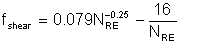
Equation 6/20 does not lend itself to an explicit solution such as could enable us progress further with our concept development. Fortunately, since a smooth pipe is assumed, and since we are dealing with liquid flow where Reynolds number is normally always less than 105, there are explicit equations that are just as good. One such equation is that proposed by Blasius, which is good for Reynolds numbers up to 105: Blasius' equation, originally given for Darcy friction factor, is expressed for Fanning friction factor thus:
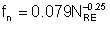
| Eqn 6/22 |
The difference between equations 6/21 and 6/22 represents the internal energy loss
The difference between equations 6/21 and 6/22 represents the internal energy loss due to turbulence within the fluid, and which therefore causes break-up of the liquid into droplets. That is, we can define
| Eqn 6/23 |
Replacing NRE with the expression for Reynolds number and rearranging the equation, we have
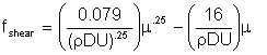
| Eqn 6/24 |
Let us attempt to relate the droplet diameter to the rate of pressure loss accountable to fluid internal friction. We will adopt the approach of dimensional consistency. First, we must insinuate what parameters we consider influencial in the process. Intuitively, we can expect the following to have an influence:
The droplet diameter has dimension L
Mathematically,
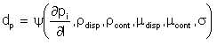
| Eqn 6/25 |
This author wishes to also suggest that what is significant in respect of densities and viscosities is the ratios of the quantities. Consequently, they will not immediately feature in the dimensional analysis. We thus rearrange the functional relationship:
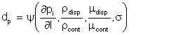
| Eqn 6/26 |
For dimensional consistency, we require that
| Eqn 6/27 |
Solution of this equation leads us to
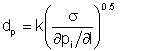
| Eqn 6/28 |
Equation 6/28 is consistent with what one would expect from physical considerations. First, froplet diameter increases with interfacial tension. Secondly, for a given point along the pipe, droplet diameter is less for higher rates of pressure loss. This is to be expected, since higher rates of pressure loss derive from faster flow velocities and therefore greater turbulence.
The effects of phase density ratio and phase viscosity ratios are intrinsic in the dimensional constant k.
We point out that, in strict sense, it is the instantaneous rate of pressure loss that applies to equation 6/28. Because the average droplet diameter varies along the pipe, viscosity of the emulsion and hence the instantaneous rate of pressure loss varies along the pipe. However, if we choose to be liberal and adopt a constant (which could well be the average) rate of prtessure loss in the pipe, then we obtain a constant droplet diameter.
Comparing equation 6/28 with Sleicher's equation (6/15), it would appear that our equation is much simpler. However, this simplicity is only apparent. The rate of pressure loss embodies several parameters - flow velocity, fluid density, and viscosity, which are individually identified in Sleicher's equation. Also, as we pointed out earlier, constant k in equation 6/28 embodies the phase densities and viscosities.