Roulette System Fibonacci ®)SelMcKenzie

Fibonacci entwickelte die nach ihm benannte Zahlenfolge, welche sich darstellt als 1-1-2-3-5-8-13-21-34-55-89-144 usw. Der Reiz der Fibonacci-Folge ist, dass sich mit ihr ein mathematisches Verhältnis beschreiben lässt. Teilt man jede Zahl durch die vorhergehende Zahl (z.B. 13 ./. 8 oder 21 ./. 13), nähert sich die resultierende Zahlenfolge asymptotisch einer konstanten Relation, welche 1,61803398875... lautet und eine irrationale Zahl ist, d.h. das Verhältnis kann niemals exact  bis auf die letzte Stelle nach dem Komma bestimmt werden. Für die Verwendung bei diesem System rechnen wir deshalb mit einem abgerundeten Fibonacci-Quotienten von 1,618. Wenn jede Zahl der Fibonacci-Folge durch die nachfolgende Zahl geteilt wird, ergibt dies einen asymptotischen Prozess, der zu der Relation PHI führt mit 0,618.  Analytisch wird diese Fibonacci-Fiolge etwas modifiziert und umgeschrieben zur PHI-Folge, die sich wie folgt darstellt: 0,618-1,000-1,618-2,618-4,236-6,854-11,090-17,944...

 Wenn wir jedes Element der PHI-Folge  durch das je vorhergehende Element teilen (z.B. 4,236 ./. 2,618 oder 6,854 ./. 4,236) erhalten wir als Ergebnis die angenäherte Relation PHI=1,618. Dividieren wir andersherum jedes Element der PHI-Folge durch das jeweils nachfolgende Element (z.B. 2,618 ./. 4,236 oder 4,236 ./. 6,854) ergibt das als Resultat den Kehrwert zur PHI als PHI = 0,618.

Bei dem Fibonacci-Quotient  handelt es sich um eine wichtige mathematische Repräsentation natürlicher Phänomene. Bei der Analyse von Permanenz-Verläufen und der Entwicklung von Strategien kann nach Strukturen und Pattern gesucht werden, die sich bisher als profitable erwiesen haben und denen deshalb eine Wahrscheinlichkeit für weitere Profitabilität zugeschrieben werden sollte. Die Fibonacci-Verhältniszahl stellt eine derartige Struktur oder solche Patterns dar.

Ein brauchbarer Weg, den Fibonacci-Quotienten in der Geometry anzuwenden, um diese Relation als geometrisches Instrument beim Roulette mittels PHI-Spiralen und PHI-Ellipsen anzuwenden, wurde von uns bisher einzig und allein publiziert („The Gemetry of Gambling“, Author Dieter Selzer-McKenzie, SelMcKenzie-Publishing) . Sowohl PHI-Spiralen als auch PHI-Ellipsen besitzen aussergewöhnliche Eigenschaften, die in zweierlei Hinsicht in Bezug zur Fibonacci-Relation PHI stehen: Geworfener Abstand in Kessel-Fächern und Links- oder Rechtsdrehung. Es ist sehr wahrscheinlich, dass die Integration  von PHI-Spiralen und PHI-Ellipsen die Interpretation und den Verwendungsnutzen der Fibonacci-Relation auf ein deutlich höheres Niveau heben wird. Fibonacci’s PHI ist ein Werkzeug zur Messung von Korrekturen und Extensionen in Wurfweiten. Die Berücksichtigung von PHI-Spiralen und PHI-Ellipsen erlauben zusätzlich die adäquate Verbindung von Kessel-Fächer-Abständen, Links- und Rechts-Drehungen in einem geometrischen Analyseansatz. 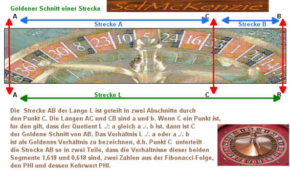PHI-Spiralen und PHI-Ellipsen basieren auf  den sogenannten Goldenen Schnitt einer Strecke bzw. dem Goldenen Schnitt eines geometrischen Körpers (hier: Roulette-Kessel).

Die Verwendung von Kessel-Fächer-Abstands-Zielen als zweites der geometrischen Fibonacci-Werkzeuge ist aus der selben Logik abgeleitet, wie die Fibonacci-Folge. Kessel-Fächer-Abstands-Ziele sind jene Kessel-Sectoren, an denen ein Ereignis auftreten könnte. Durch Multiplikation des Abstandes von Punkt A zu Punkt B (oder jeder anderen Abstands-Messung) mit der Fibonacci-Relation wird errechnet aus dem Wendepunkt C als C=B+1,618x(B-A). Punkt C wird als Fibonacci-Abstands-Ziel bezeichnet.

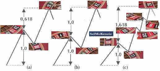
Ziel-Korrekturen und Ziel-Extensionen sind die dritte Kategorie des geometrischen Fibonacci-Instrumentes. Der gängigste Ansatz zur Definition der Ziel-Korrektur erfolgt über die Anbindung  der Grösse der Ziel-Korrektur  an einem Prozentsatz einer vorhergegangenen Impulsbewegung dieser Abstands-Messung. Bei der Analyse interessieren drei ausgewiesene Prozentsätze, die unmittelbar aus der Fibonacci-Folge und den Quotienten der PHI-Folge abgeleitet werden können, und zwar 38,2% ist das Resultat der Division 0,618 ./. 1,618, 50,0% ist die Transformation des Verhältnisses 1,000, 61,8% ist die unmittelbare Fibonacci-Relation 1,000 ./. 1,618.

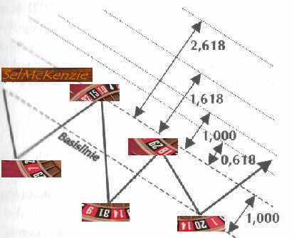
PHI-Kanäle, als viertes Instrument in unserem geometrischen Instrumentensatz, werden generiert durch die Zeichnung von parallelen Linien durch Abwurf-Event und Zielwurf-Event. Die Weite des PHI-Kanals wird berechnet als Distanz  zwischen Base und Parallele. Diese Distanz wird gleich 1,000 gesetzt. Weitere Parallelen ergeben sich im PHI-Folge-Abstand, beginnend mit 0,618-mal der Abstand des PHI-Kanals, dann 1,000-mal, 1,618-mal, 2,618-mal, 4,236-mal usw. der Distanz zwischen Base und Parallele.

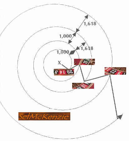
PHI-Spiralen, als fünftes Instrument stellen die optimale Verbindung zwischen Base und parallele dar. Geometrisch ist die Grösse der PHI-Spirale determiniert durch den Abstand zwischen dem Zentrum X der Spirale und dem Startpunkt A (Abwurfpunkt). Die PHI-Spirale dreht entweder je nach Kessel-Drehung nach links oder rechts, um die Basislinie, die vom Zentrum der Spirale zum Startpunkt läuft. Während die PHI-Spirale wächst, dehnt sie sich mit einer konstanten Rate bei jeder vollen Umdrehung aus. Alle diejenigen Spiralen, welche mit Raten wachsen, die Elemente der PHI-Folge 0,618-1,000-1,618-2,618-usw. sind, sind als PHI-Spiralen für die jeweilige Satz-Berechnung anzuwenden.

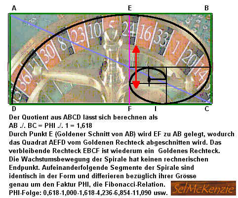
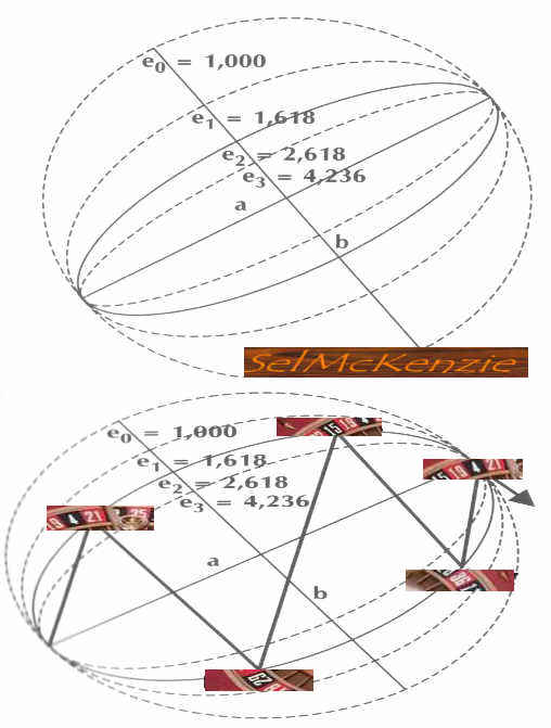
PHI-Ellipsen sind das sechste Instrument. Eine Ellipse wird zu einer PHI-Ellipse in allen Fällen, in denen der Quotient aus Hauptachse und nebenachse der Ellipse ein Element der PHI-Folge 0,618-1,000-1,618-2,618-usw. ist. Ein Kreis ist in diesem Sinne eine spezielle PHI-Ellipse, für die gilt: a=b (Quotient a ./. b = 1).

Anwendung der speziell von SelMcKenzie entwickelten bzw.veränderten Indicatoren bzw. Oszillatoren:

Coppock: 
Der Coppock misst langfristige Trends, in dem zwei langfristige Momentums addiert werden. Auf Basis dieser Summe wird ein gewichteter Gleitender Durchschnitt der gefallenen Kessel-Fächer-Abstands-Längen gebildet. Da die Basis des Indikators vom Momentum gebildet wird, oszilliert auch der Coppock um die Zeroline.
Formel/Berechnung
Coppock = WMAx(ROCy + ROCz)
wobei:
WMA = Weighted Moving Average 
Der Coppock wird auf zwei verschiedene Weisen interpretiert. Standard ist die Drehung des Kessels oberhalb der Zeroline nach unten als Mass-Signal, die Drehung der Linie unterhalb der Zeroline nach oben als Conform-Signal zu interpretieren.

Envelopes:
Für die Envelopes wird ein Gleitender Durchschnitt der gefallenen Kessel-Fächer-Abstands-Längen berechnet, auf Basis dessen zwei (obere und untere) Bänder berechnet werden. Der Abstand der Bänder vom Gleitenden Durchschnitt der gefallenen Kessel-Fächer-Abstands-Längen ist in der Regel identisch. So wird ein Grossteil der satzreifen Pleins in einem Envelope eingefangen.

Gleitender Durchschnitt Kessel-Fächer-Abstands-Längen:
Der Gleitender Durchschnitt der Kessel-Fächer-Abstands-Längen drückt die beiden wichtigsten Eigenschaften des Indikators aus. Durchschnitt heisst, dass über eine bestimmte Anzahl von Coups ein Mittelwert der gefallenen Kessel-Fächer-Abstands-Längen gebildet wird. Gleitend drückt aus, dass die Berechnung mit jedem neuen Coup um eine Coup-Messung nach vorne verschoben wird, der bis dahin letzte Coup fällt also aus der Berechnung hinaus. Die Mittelwert ist natürlich im wahrsten Sinne des Wortes trendfolgend, daher ist der Gleitende Durchschnitt Kessel-Fächer-Abstands-Längen ein wichtiger Trendfolger.

Gleitender Durchschnitt Weighted Kessel-Fächer-Abstands-Längen:
Bei dieser Berechnung werden alle Kessel-Fächer-Abstands-Längen nochmals mit einem Gewichtungsfaktor versehen. Im allgemeinen werden die Factoren mit zunehmender Nähe der Coups grösser. So wird erreicht, dass die aktuelleren Coups mit einer höheren Gewichtung in die Satz-Findung einfliessen.

Momentum:
Das Momemtum versucht die Kraft eines geworfenen Fach-Abstandes zu messen, indem von der Länge des letzten Coups einfach die Längen von vor einigen Coups abgezogen wird. Der Indikator-Verlauf schwankt damit um die Zeroline.. Sinn dieser Subtraktion ist das Erkennen neuer Trends, die sich häufig durch große Abstands-Bewegungen zu etablieren versuchen. Im Laufe des Trends lässt die Kraft, und damit der absolute Wert des Momentums, häufig nach.
Anstelle der Subtraktion der Coup-Längen können Sie die beiden Kurse auch dividieren, die Aussage bleibt identisch, lediglich die Basislinie ändert sich. Ein Momentum im negativen Bereich deutet immer auf ein Negativum hin, fällt das Momentum zusätzlich weiter, so nimmt die Kraft des Negativum noch weiter zu. Ein steigendes Momentum unterhalb der Zeroline deutet auf eine Abschwächung des Negativums hin - und damit auf einen eventuell anstehenden neuen, gerichteten Trend zum Positivum.
Eine weitere Anwendung ist die Suche nach Divergenzen zwischen Permanenzverlauf und Momentum. Bildet das Momentum noch neue Divergenzen, der Basiskurs aber nicht mehr, so können Sie mit einem baldigen Trendwechsel rechnen.

Moving Average Convergence Divergence Indikator:
Der Moving Average Convergence Divergence Indikator, im folgenden nur noch MACD genannt, hat sich um Laufe der letzten Jahre zu einem der am meisten verwendeten technischen Indikatoren entwickelt. Besonders interessant ist an diesem Indikator, dass er aufgrund seiner Berechnung und Interpretation in nahezu jeder Coup- bzw.Permanenz-Lage zu verwenden ist. Von daher ist er im Prinzip sowohl als Trendfolger als auch als Oszillator zu bezeichnen - seine Basis, 3 Gleitende Durchschnitte Kessel-Fächer-Abstands-Längen deuten auf jeden Fall, auf den trendfolgenden Charakter hin.
Der MACD an sich subtrahiert 2 Gleitende Durchschnitte Kessel-Fächer-Abstands-Längen voneinander. Allerdings werden diese beiden Gleitende Durchschnitte Kessel-Fächer-Abstands-Längen immer auf exponentieller Basis berechnet. Der Verlauf oszilliert also um die Zeroline. Eine Feststellung oberhalb der Zeroline zeigt an, dass der kurze Gleitende Durchschnitt Kessel-Fächer-Abstands-Längen oberhalb des langen Gleitenden Durchschnitt Kessel-Fächer-Abstands-Längen liegt, eine Ermittlung unterhalb der Zeroline drückt damit das genaue Gegenteil aus.
Die im Namen enthaltene Konvergenz / Divergenz Betrachtung kommt durch Auswertung des Abstands Zeroline und MACD-Verlauf zum Tragen, je weiter die Linie von der Zeroline von der Zeroline entfernt ist, um so stärker ist die Divergenz. Eine wachsende Divergenz deutet auf eine Intensivierung des vorherrschenden Trends hin, eine Abnahme auf eine Schwächung des Trends. Entscheidend ist also die Trendwende in der MACD-Line. Um diese in den Griff zu bekommen, haben wir eine zweite Linie, einen Gleitenden Durchschnitt Kessel-Fächer-Abstands-Längen von der MACD-Line, eingeführt. Die Signale werden daher beim Schnitt dieser Linie mit der eigentlichen MACD-Line generiert.
Eine etwas schwierigere Anwendung ist die Verwendung des MACD zur Untersuchung von Divergenzen mit der Basisline. Schwieriger deshalb, weil Sie in diesem Fall selbst Trendlinien errechnen müssen, um zu einem Ergebnis zu kommen. Ein Beispiel wäre das Herausbilden neuer Coup-Fach-Abstände im Basiswert, während die Coup-Fachabstände im MACD schon zurückgehen - in diesem Fall ist mit einer baldigen Trendumkehr, also dem Fallen des Basisline zu rechnen.

On-Balance Volume:
Der On-Balance Volume Indicator, abgekürzt mit OBV, setzt Volumen (Coups) und Fach-Abstands-Längen-Veränderungen in Relation. 
Der OBV-Indicator addiert bzw. subtrahiert das Volumen des Wertes für eine gegebene Periode abhängig davon, ober der letzte Coups bzw. deren Fach-Abstand höher oder niedriger als der Vorletzte ist. Der OBV wird meist noch geglättet.

Rate of Change:
Das Rate of Change, abgekürzt mit ROC, liefert im Prinzip genau die gleiche Aussage wie das Momentum. Aufgrund seiner etwas anderen Berechnung kann es aber bei der Generierung dieser Anwendung eventuell sinnvoll sein, anstelle des Momentum das ROC einzusetzen. Wie bereits angedeutet, bietet das Rate of Change vielfältige Anwendungsmöglichkeiten. Im folgenden beschreiben wir Ihnen die wichtigsten Grundlagen, auf denen Sie dann Ihre Ideen aufbauen können.
Ein Rate of Change im negativen Bereich deutet immer auf einen Gegentrend hin, fällt das Rate of Change zusätzlich weiter, so nimmt die Kraft der Gegentrendbewegung noch weiter zu. Ein steigendes Rate of Change unterhalb der Zeroline deutet auf eine Schwächung des Gegentrends hin - und damit auf einen eventuell anstehenden neuen, positiv gerichteten Trend.
Ein positives Rate of Change zeigt einen paritätischen Trend an, ein steigendes ROC in diesem Bereich deutet weiterhin auf eine Verstärkung des paritätischen Trends hin. Fällt das Rate of Change, so könnte der paritätische Trend bald dem Ende zugehen. 
Das klassische Signal liefert der Durchbruch der Mittelpunktslinie. Von unten nach oben ist es ein Satz-Signal, von oben nach unten kein Satz-Signal. Um Fehlsignale zu vermeiden, können sich auch zwei nach oben oder unten angesetzte Hilfslinien einzeichnen. Ein Signal soll in diesem Fall erst dann Gültigkeit haben, wenn eine dieser Hilfslinie durchbrochen wird.
Eine weitere Anwendung ist die Suche nach Divergenzen zwischen Permanenzverlauf und Rate of Change. Bildet das Rate of Change noch neue lange und kurze Abstands-Weiten, die letzten Coups aber nicht mehr, so können Sie mit einem baldigen Trendwechsel rechnen.

Relative Stärke Index nach SelMcKenzie:
Der Relative Stärke Index nach SelMcKenzie gehört, zusammen mit dem Gleitenden Durchschnitt Kessel-Fächer-Abstands-Weiten und dem Momentum, zu den am häufigsten gebrauchten Indikatoren für die Anwendung dieses Systems.
Der RSI versucht die innere Stärke als die Entwicklung des voraussichtlichen Permanenz-Verlaufes innerhalb einer bestimmten Anzahl von Coups zu messen. Im RSI wird ein Verhältnis zwischen den Kessel-Fächer-Wurf-Längen der jeweiligen Coups gebildet. Der Indicator selbst schwankt aufgrund der Formel immer zwischen 0 und 36. Der Vorteil dieser Vereinheitlichung liegt darin, dass einzelne Werte so gut verglichen werden können. Durch die Einbeziehung aller Coups innerhalb des Permanenz-Verlaufs erreicht man auch eine gewisse Glättung, Extrem-Ausschläge im Permanenz-Verlauf verzerren also die Berechnung nicht mehr so. 
Erreicht der RSI 0 (Zero), so hat der Verlauf keinerlei innere Stärke. Die Coups sind also im Betrachtungszeitraum ausschliesslich unwesentlich. Ein Wert von 36 bedeutet, dass die Coups ausschliesslich poistiv für die Satz-Feststellung sind. Werte in der Nähe von 0 (Zero) deuten auf einen negativen Satz-Erfolg, Werte in der Nähe von 36 auf einen poistiven Satz-Erfolg hin. An solchen Punkten können Sie mit einer Umkehr des Verlaufs rechnen. Das echte Signal wird allerdings erst dann erzeugt, wenn der Indicator den Extrembereich um das Minimum bzw. Maximum wieder verlässt.

Smoothed Rate of Change:
Das Smoothed Rate of Change, abgekürzt mit SROC, und stellt eine Abwandlung des Momentums bzw. des ROC dar. Beim SROC wird anstelle des Permanenzverlaufs allerdings ein Exponentieller Gleitender Durchschnitt Kessel-Fächer-Abstands-Längen als Grundlage für die Berechnung verwendet.
Dies entspricht weitestgehend der des Momentums, mit dem Unterschied, dass die Satz-Signale etwas weniger, aber auch etwas treffsicherer kommen.
Die Interpretation des SROC folgt den Regeln des Momentums, besonders interessant ist die Suche nach Divergenzen zwischen SROC- und Permanenz-Verlauf. Ein negatives Satz-Signal ist dann gegeben, wenn der letzte Coup noch neue Abstands-Längen ausbildet, während der SROC keine neuen Längen mehr bildet, ein positives Signal ist dann gegeben, wenn umgekehrt. 

Time Series Forecast:
Der Time Series Forecast (TSF) ähnelt einen Gleitenden Durchschnitt Kessel-Fächer-Abstands-Längen, da auch er versucht, den Trend eines Permanenz-Verlaufs anzunähern. Der Hintergrund dieses Indicators ist im Gegensatz zu vielen anderen Indicatoren nicht sehr einfach, sondern eher etwas anspruchsvoll.
Die Trendmessung erfolgt nicht in Form einer Glättung (siehe Gleitender Durchschnitt Kessel-Fächer-Abstands-Längen), sondern dadurch, dass über den Permanenz-Verlauf sogenannte Regressionsgeraden, die die Steigung an genaue einem Coup des Permanenz-Verlaufs messen, berechnet werden. 
Es bieten sich zwei verschiedene Interpretationsmöglichkeiten an. Zum einen der Schnitt des TSF mit einem auf ihn berechneten TSF. Ein Satz-Signal ist gegeben, wenn der TSF seinen Gleitenden Durchschnitt Kessel-Fächer-Abstands-Längen von unten nach oben schneidet, kein Satz-Signal dann, wenn der TSF seinen Gleitenden Durchschnitt Kessel-Fächer-Abstands-Längen von oben nach unten schneidet.
Die andere Möglichkeit ist die, den Schnitt des TSF mit dem letzten Coup zu untersuchen. Ein Satz-Signal ist gegeben, wenn der Abstand den TSF von unten nach oben schneidet, kein Satz-Signal dann, wenn der Basiswert den TSF von oben nach unten schneidet.

Trend-Bestätigungs-Indicator:
Der Trend-Bestätigungs-Indikator, abgekürzt TBI, basiert auf zwei gleitenden Durchschnitten der Kessel-Fächer-Abstands-Längen.
Der TBI versucht einen bereits durch einen Gleitenden Durchschnitt Kessel-Fächer-Abstands-Längen erkannten Trend mit Hilfe eines zweiten Gleitenden Durchschnitt Kessel-Fächer-Abstands-Längen zu bestätigen. Die beiden Gleitende Durchschnitte Kessel-Fächer-Abstands-Längen werden dazu dividiert. Die so erhaltene Kennziffer schwankt somit um die Zeroline.
Ein Satz-Signal liefert der Indicator, wenn der Verlauf die Zeroline von unten nach oben schneidet. Dies bedeutet, dass der kürzere Gleitende Durchschnitt Kessel-Fächer-Abstands-Längen den längeren überholt, also von unten nach oben geschnitten hat. In diesem Moment ist der durch den längeren Gleitenden Durchschnitt Kessel-Fächer-Abstands-Längen definierte Trend von dem kürzeren Gleitenden Durchschnitt Kessel-Fächer-Abstands-Längen bestätigt worden. Umgekehrt, also bei einem Schnitt der Zeroline von oben nach unten, gilt spiegelbildlich das gleiche.

Gamblers can typically describe the methods they use to initiate and liquidate trades. However, when forced to describe a methodology for the amount of capital to risk when trading few traders have a concrete answer. Some make vague references to experts that recommended risking one or two percent of portfolio equity on any trade. Others rely on intuition to determine when to increase position size on a particular trade, always risking different amounts. 

Experienced traders learn, however, that as important as it is to have an effective method to determine when to trade, it is equally important to develop a methodology to determine how much to risk. A trader that risks too much increases the chance that he will not survive long enough to realize the long run benefits of a valid trading strategy. However, risking to little creates the possibility that a trading methodology may not realize its’ full potential. 

Therefore, while a positive expectation may be a minimal requirement to trade successfully, the way in which you are able to exploit that positive expectation will in large part determine your success as a trader. This is, in fact, one of the greatest challenges for traders. 

At SelMcKenzie-Systems-Software, we have had the fortune of working with many experienced traders, and in that process we became increasingly aware of the need for sound methods for applying money management strategies. In fact, it seems that as traders reach a certain level of comfort with a system they begin to realize that a sound money management approach is missing from their trading strategy. Our work in this area has led us to research several strategies for determining position size and ways in which to add to, decrease, and stop out positions. Many of these strategies are well known and readily available in the public domain and others are hybrids that we have built from improving concepts already available. Moreover, once you understand the importance of money management, the opportunity to modify many of the well-known strategies to meet your needs is endless. 

It is our belief that there is really no “black box” formula for money management. That is, different trading strategies and systems require different approaches to money management. In addition, we must always consider the trader’s ability to implement a money management strategy given their tolerance for risk and other psychological factors. For example, several strategies that emphasize optimizing the amount of capital to invest in a trade to achieve maximum returns often deliver substantial drawdowns. Few traders are comfortable suffering through a drawdown of fifty, sixty, or seventy percent, which is not unheard of for some aggressive strategies. Therefore, it is essential to match the theoretical drawdown with the traders ability to tolerate it. 
Finally, and not insignificant, is that a trader’s capitalization may effect their ability to execute a strategy. Even in cases where it might be preferable from a system performance perspective to utilize a money management strategy that tends to add to positions as the price moves against the trader, an undercapitalized trader may be unable to add to positions during a drawdown in equity while in a trade. In this situation the trader would be unable to derive the potential benefits of the strategy. 
Therefore, apart from the effectiveness of a particular strategy on a given trading methodology, there are two important variables: the psychological preferences of the trader and their level of capitalization. If either of these two factors do not support the money management strategy employed, then it is unlikely the trader will be able to use the strategy effectively. Though seemingly insignificant, this point cannot be overemphasized because as many strategies are developed over large histories of data (in many cases 10 or 20 years of data). The trader needs to have the confidence to remain with the strategy even if positive results do not come immediately. 
We believe that you will benefit from the strategies presented in this guide. In addition, we hope we have created a greater awareness for the need to evaluate what type of money management system you are using. Hopefully, we will spur your imagination when thinking about ways in which to use money management. We find that many traders focus much of their creativity on entry and exit logic. However, a range of methods for determining position size can be employed and traders are well advised to devote considerable effort in determining this as well. 

It should be noted that all traders are using some form of money management. Some, though, are not conscious of what type of strategy or method they are using. Other traders use thought out and tested methodologies for determining how much capital to commit to trades and sound strategies for adding to or exiting positions which are consistent with their expectations of risk. It is our hope that you will find yourself among the latter group.

Introduction: 
The goal of this book is to explain the process by which traders can develop, evaluate and ultimately improve the performance of trading systems with money management strategies. These improvements must be based on an individuals risk tolerance and trading psychology. At SelMcKenzie-Systems-Software we have developed an evaluation and improvement process to address these issues. 
We believe that money management does not exist in a vacuum. This means that it is essential that your money management strategy be integrated into an overall approach to system design and development. Therefore, before we move directly into the application of various money management strategies we will focus on some elementary issues concerning system design and testing. We believe this is an essential component in our approach to money management. To provide you with an adequate foundation to apply money management we will take you through the necessary stages of development that precede the application of money management. It is a requirement that the trader sufficiently understands the methodology being employed and where its’ likely to succeed or fail. 
To assist in our evaluation we will present analysis that has been derived using MoneyManager and 3D SmartView from SelMcKenzie-Systems-Software and Portfolio Maximizer. 
While many approaches and strategies to money management are available, in this book we will focus on the money and risk management strategies listed below:Maximum Adverse Excursion
Maximum Favorable Excursion
Drawdown Support
Winning Series
Fixed FractionalOptimal f
Secure f
 
In addition, we will combine some of these strategies to create a fully integrated approach to money and risk management. Once again, we do not claim nor intend to cover all of the strategies for money and risk management available to traders. We do, however, strive to present a useful overview of several techniques available to traders to achieve effective money management methodology. 
 
Before we get into the details, let’s take this opportunity to briefly discuss the chapters we will cover in this book. 
In chapter one we will design a methodology to trade the currency markets using continuous price data. In addition, we will center on developing and programming the system using TradeStation by Omega Research. It should be noted, however, that many of our examples could also be implemented in Microsoft Excel or other spreadsheet applications. 
In chapter two we will begin evaluating the stability of our trading system. We will use three dimensional graphs to help evaluate the robustness of our Euro trading system. Once again, this type of analysis can be accomplished using a variety of spreadsheet or advanced mathematics packages available. 
In chapter three we will evaluate the systems’ performance to determine if the trading characteristics of the system fit our psychological profile. We will use Portfolio Maximizer, an evaluation package co-developed by SelMcKenzie-Systems-Software and Research, to assist in our detailed system evaluation. This detailed evaluation will be invaluable as we begin applying our money management strategies. 
The process of improving the performance of the system by applying money, risk, and equity management strategies is addressed in the fourth chapter. We will build on the evaluation stage by testing a number of money and risk management techniques to determine which strategies work best with our system. This stage is critical to making significant improvements to the performance of our Euro system. 
In chapter five we will conclude our discussion of money management by analyzing the performance of our portfolio to ensure that a risk-adjusted portfolio is created. Issues relating to diversification and the way systems interact in a portfolio are discussed. 
In summary we will design a simple trading system, evaluate its performance and ultimately improve its results using a variety of money management strategies. 
Although the focus of this book is on money management, it is important to realize that it is imperative that know as much about our system as possible to justify applying specific money management strategies. This implies that we fully evaluate our systems design and performance prior to applying any form of money management. Once the evaluation is complete we can apply appropriate money management strategies with a high degree of confidence that our systems performance results will be improved in accordance with our risk tolerance.
System Design:The goal of Elements of Money Management is to introduce and apply a systematic process of developing, evaluating and improving trading systems. Once you understand this process you can apply it to any number of systems or trading ideas you may have. 
The sample system we have selected is a simple moving average crossover system that trades the Euro. If we are able to design a profitable system using this methodology then imagine what you can do with more complex trading systems and methodologies. By using a simple system in particular, we do not have to spend a lot of time on the system itself, but rather we can spend our time on the process of evaluation and improvement, which is, after all, the goal of this book. 
Our base system, once taken through the evaluation and money management process will generate superior performance, especially or such a simple system. The actual improvement will increase the system‘s net profit by over 635%. This is a huge increase given the fact that we are designing a simple Moving Average trading system. The net result will be a stable system that is highly profitable and easy to trade. 
The first step in designing a system is to evaluate what type of market we are trading. Markets basically come in two types; Trending and Non-trending. Each of these markets will have their own personality.

Trending vs. Non-Trending : 
Trending markets have a tendency to move in the same direction for extended periods of time in either a bullish and bearish manner. The currencies are an example of markets that often exhibit this trending behavior. To illustrate this lets look at a graphic of a trending market. 
Exhibit 1:Trending Notice that once the market begins its trend it typically moves in the same direction for a long period of time. Trending markets are typically traded with breakout or moving average systems. This type of systems never catches the exact top or bottom of a market, but rather it aims to remain with the general trend. Trending systems do not necessarily generate a lot of winning trades, but when they experience a profitable trade it is typically quite large. 
Non-trending like the financials have a tendency to make quick moves reversing direction at the drop of a dime. Our next exhibit illustrates a non-trending market. 
Exhibit 2: Non-Trending  Notice how the market appears to be locked between support and resistance levels. These levels help determine when the market is overbought or oversold. Non-trending markets are typically traded with momentum indicators such as RSI, %R, CCI as well as whole host of other rate-of-change based indicators. These systems attempt to catch the tops and bottoms and are typically have a higher percentage of winning trades than trending systems. Non-trending systems are capable of generating a large number of consistent profitable trades. 
By reviewing the underlying market we can determine whether it’s trending or non-trending. Now bear in mind that all markets whether they are futures, stocks or mutual fund exhibit signs of being both trending and non-trending. So what we are talking about here is the markets primary nature -- is it typically trending or non-trending? Once we know what we are dealing with developing our primary system is a lot easier and a great deal more profitable. 
We are attempting to ensure that our methodology is consistent with the behavior of the underlying market. Attempting to use a long-term trend following system on a choppy market generally does not work. It is for this reason that every system may not be appropriate for every market. 
Since we will be trading the Euro, we will want to design a system that is primarily trend following oriented. The system will be based on a simple moving average crossover that will attempt to capture the majority of the larger trends in the Euro. 
Now that we know a little more about the trading characteristics of our market we are ready to develop the trading system. 
 
CrossOver Methodology:We begin with the typical crossover system that goes long the market when the faster moving average crosses the slower moving average. The system remains long until the moving average crosses in the opposite direction causing the system to short the market. 
Let’s take a look at a graphic to better understand our trading logic. 
Exhibit 3: Crossover Methodology 
 
The system goes long at point A where the moving averages cross in a positive manner. And at point B the system reverses and goes short as the moving averages cross again in a negative manner. The system initiates a new trade every time the moving averages cross one another. 
This basically describes our trading methodology but already there is a conceptual flaw that will effect the long-term performance of our system. This flaw centers on how the system trades the long and short side of the market. 
 
Greed and Fear DescriptionLet’s explain the need to develop a methodology for both the long and short side in a little more detail. No matter which market you trade, all markets are effected by human nature; greed and fear. Markets have a tendency to move in a direction for an extended period of time and then quickly reverse. The greedy nature of traders accounts for market trending in a certain direction whether it’s bullish or bearish. Fear on the other hand accounts for the quick reversal of fortune. When the herd mentally of the market decides to change direction it may do so very quickly. Greed and fear help to explain why markets react the way they do to bull and bear moves. These bullish and bearish tendencies can be seen in all time frames whether they are short or long term. What is important to realize is that trading boils down to human nature; greed and fear. 
If the markets are effected by greed and fear then so too is the system. The conceptual flaw in our system relates to the fact that our system trades long then short and then repeats again. Any time the moving averages cross one another we reverse our position. A reversal system that trades 100% of the time doesn't give us any opportunity to make adjustments at the system development stage. And for that matter, it will really effect us at the money management stage. 
Because we want to design an effective trading system -- we will have to account for greed and fear in the development of our system. To do this we will develop two systems to trade the same market. One only goes long and the other short. Splitting the methodology into two systems allows use to evaluate and improve the individual systems and then combine them back together at the portfolio level. Developing systems separately for both the long and the short side gives us greater flexibility in evaluating and improving our system. 
 
System Development Process: 
We now have one more refinement to properly develop the trading system. This involves separating the entry and exit signals. There is no reason to believe that whatever logic got us into our trade is appropriate to exit the trade. Let's take a look at Exhibit 4 to see exactly how we are developing our system. 
Exhibit 4: System Development Process 
 
Whenever possible we want to bring our system down to the lowest level, which in this case is the signal level. We have entry signals and exit signals for both our long system and short system. The entry and exit signals combine to create our separate long and short systems. These two separate systems are then combined to create our mini portfolio. The net result is -- we end up with a system that trades long and short but allows us to refine the system based on our robustness analysis, system evaluation and money management strategies. 
 
System Code: 
Let's take a look at the code to our system to better understand how it trades. For the sake of time we will focus primarily on the Long side. 
Exhibit 5: Long Moving Average Crossover SystemInput: Length1(8),Length2(20), Length3(5),Length4(23);
 
IF CurrentBar > 1 and Average(Close,Length1) crosses over Average(Close,Length2) Then Buy on Close; 
IF CurrentBar > 1 and Average(Close,Length3) crosses below Average(Close,Length4) Then Exitlong on Close; 
We see that our system enters into a Long position when the Moving Average #1 crosses over Moving Average #2. The position is exited when Moving Average #3 crosses below Moving Average #4. 
This system is very similar to every moving average system ever developed. We simply go a step further by breaking the system down to a lower level. Therefor we have four inputs per system. As you can see at the top of Exhibit 5 the system inputs are Length 1 through Length 4 which correspond to the four moving averages. The short trading system shown below follows the same logic using separate moving averages to enter and exit its short positions. 
 
Exhibit 6: Short Moving Average Crossover SystemInput: Length1(5),Length2(20), Length3(12),Length4(15);
 
IF CurrentBar > 1 and Average(Close,Length1) crosses below Average(Close,Length2) Then Sell on Close; 
IF CurrentBar > 1 and Average(Close,Length3) crosses over Average(Close,Length4) Then ExitShort on Close; 
In summary, we have separated the long and short positions and refined the system by separating the entry and exit signals. These refinements will allow us to better evaluate the performance of the system. As you will see this is a key part to developing a profitable well designed system. 
 
Robustness Analysis:Robustness analysis allows us to take the inputs for a system and evaluate them to determine the most stable settings. To accomplish this task we must optimize the system inputs in TradeStation. Our goal is not to optimize our trading system to generate the largest historical net profit, but rather use the optimization report to determine the stability of our system. An unstable trading system may appear to be historically sound, but eventually the system will fail due to subtle changes in the market over time. Therefore the more stable the system over a range of inputs, the more likely it is to maintain its performance in the future. 
To help us assess our systems’ stability we will look at a variety of three-dimensional performance graphs. A few of the more important performance characteristics to consider are net profit, profit factor, the ratio of average wins to average loss and drawdown. With robustness analysis we are able to understand our system’s stability across all of these performance measures. 
If we find that the system's net profit, for example, drops off dramatically by making a small change to the input value, then we know that the system is not very stable and may be susceptible to failure in the future. If, however, the systems’ performance is NOT highly sensitive to the systems’ settings, that is, small changes in inputs do not result in a large change in the net profit then we may feel more comfortable with the stability of the system. The point is that it’s preferable to have a system perform well over a large range of values. 
Let's review the results of a trading system to better understand how to determine the robustness of a system. The system we are about to evaluate is not our moving average system but rather another system that allows us to easily see the difference between stable and non-stable trading results. Once we know what a bad system looks like it is easier to appreciate our stable Euro system. 
Exhibit 7: Unstable System 
The results in Exhibit 7 reflect the net profit output for a trading system plotted on a three-dimensional graph. The system has been optimized generating a Net Profit figure for each of the system’s inputs.  Notice the rounded Net Profit section on the right hand side of the graphic. Any small adjustment made to the system’s inputs has little effect on the net profit. The system's net profit ranges between Euro41,000 and Euro43,000. This amounts to less than a 5% deviation. 
The left-hand side of the 3D SmartView graphic tells a different story. The system's net profit figure drops off dramatically with little adjustment made to the system's inputs. The system's optimized net profit figure generated a Euro54,000 net profit. But a slight adjustment to the inputs produces a net profit figure of Euro34,000 in one direction and Euro22,000 in another. That's a 40% and 63% decline in profitability, respectively, based on a small adjustment to the systems inputs. 
We would hate to be trading this system with parameters set at the spike. The likely hood that the system will continue to trade at that level is very low. Selecting the inputs on the right hand side of Exhibit 7 will produce less of a historic net profit, but a much more stable system for trading in the future. 
The bottom line is, the system is stable, with certain input settings and very unstable with other settings. Evaluating your system using three-dimensional area graphs of a system’s performance over a range of parameters is a tremendous aid in evaluating the robustness of your trading system. 
 
Optimization pro’s and con’s 
Optimization can be your best friend or worst enemy. It all depends upon how you use it. Because it is often used incorrectly, optimization has a bad reputation. However, instead of using it to make the system look better from a historic perspective, we should use it to evaluate a system’s sensitivity to changes in the underlying market. 
It’s always surprising when traders say that they don't use optimization because they don't want to fit their system to past data. Without analyzing the robustness of a system how do they know they haven’t inadvertently selected highly unstable system parameter settings. Traders may make a conscious effort not to “fit” the data but through lack of testing actually DO fit their system to the past. Performing a simple robustness analysis on a system will go a long way to ensuring that curve fitting is minimized.  
Cluster Analysis:We want to recognize, of course, that Net Profit is an important performance measure, however, we should also pay attention to several other measures of performance. Robustness analysis involves reviewing the results of a number of performance related statistics including profit factor, percent profitable trades, the ratio of average wins to average losses, maximum drawdown, and several others. The goal is to find an area that offers stable trading results simultaneously across several system performance measures and several inputs. We call this process cluster analysis. 
Let's return our attention to our Euro system and implement what we have just learned. 
 
Exhibit 8: Stable System based on Net Profit 
Notice that our Euro system generates stable results in the center of the graphic. If we were to evaluate the same system using all of our other performance measures they would all point to the same area. Take a look at our average trade 3D Graphic to refine our robustness analysis. 
Exhibit 9: Stable System based on Average Trade 
 
Based on our robustness analysis we have selected the following inputs for our Euro trading system. 
Long Moving Average Crossover System InputsInput: Length1(8),Length2(20), Length3(5),Length4(23);
 
Short Moving Average Crossover System InputsInput: Length1(5),Length2(20), Length3(12),Length4(15);
  
Summary:Having used three-dimensional graphs to determine robust trading inputs we can now move on to the next chapter and evaluate the performance of our system with a higher degree of confidence.
 
 System Evalution:Performing a system evaluation is critical to the design and development of a trading system. Traders need to assess their system's true performance in order to build confidence in the system. 
The rationale for a detailed evaluation is simple -- every trader has his or her own idea as to what makes a great trading system. A system that is preferable to one person may not be appropriate for another. It's not uncommon to hear two traders talk about the same trading system that one loves and the other hates. This difference of opinion is most likely attributed to their individual trading style. For example, one trader may be aggressive while the other is conservative. Because a system is historically profitable, doesn't necessarily mean that the system is suited to that trader. 
At SelMcKenzie-Systems-Software we talk to a lot of traders that say "I know my system is good because it makes money". That factor alone may not be indicative of a system that is compatible with your trading style. The reality is a conservative trader will likely not be able to tolerate the volatility that is inherent with many aggressive strategies. As well, an aggressive trader my not have the patience to remain with a conservative system. Both systems may be profitable, but just not suited to that particular trader. Understanding how you relate to your trading system is perhaps the most important element in trading. 
One factor you will want to keep in mind is that we have the ability to adjust how aggressive or conservative a system is through the use of money management. Therefore, it is not always necessary to think about whether the system is aggressive or conservative in the development stage. What we do need however is a well-designed and stable trading system to be able to subsequently improve it with money management. 
It is for this reason we perform a thorough and complete evaluation to assess the strengths and weakness of a system BEFORE we trade it. The better prepared an individual is to trade; the better chance they have of becoming a successful trader. In the end it is up to the individual to decide if the system is worth trading. No matter how profitable a system appears, if they don't have the ability to stick with the system during periods of poor performance or sufficient capital to survive drawdowns, then they should look for another system to trade. There are plenty to choose from – the goal is find the one that is most correct for the individual. 
The remainder of this chapter will concentrate on the evaluation tools offered in Portfolio Maximizer. The performance statistics presented in Portfolio Maximizer are divided into a number of sections. Each section dissects the system's performance from a different perspective. 
Evalution Process:The evaluation process begins with a general overview of the system's performance. We then begin to focus on specific areas of performance, from which we can make improvements. The entire evaluation process is comprised of the following sections.System Analysis
Total Trades
Profit Ratios
Outlier Trades
Return Figures
Drawdown/Run-up
Trading Summary
Consecutive Trades
Equity Curve Analysis
Time Analysis
 
Maximum Adverse Excursion: 
Before we begin evaluating our Euro system we must apply some form of stop logic to ensure the safety of our trading capital. The process we will use to find and set appropriate stop levels is called Maximum Adverse Excursion or MAE for short. This process was introduced to traders by John Sweeney of Technical Analysis of Stocks and Commodities magazine, and is a great tool for finding appropriate levels to place stops. 
MAE allows us to evaluate our systems’ individual trades to determine at what dollar or percentage amount to place our protective stop. Let’s take a look at how to use the MAE graphic to properly place our stop. 
Exhibit 10: Maximum Adverse Excursion 
 
This graphic shows all 59 trades that make up our system. For each trade we can see the amount of drawdown that occurred in relation to realized profit or loss. The winning trades are shown as up arrows and the losing trades are represented as down arrows. Since we are using this graphic to determine where to place our stops we have put all the winning and losing trades on the same cluster graph. So this means that although trades A and B appear to be similar they are in reality quite different. Trade A had a drawdown of Euro600 before recovering to net a profit of Euro1000. Trade B, on the other hand, had a drawdown of Euro1,250 before recovering a little to loose Euro1,000. Both Trades A and B appear to generate the same profit, when in reality the Trade A actually made Euro1,000 and Trade B actually lost Euro1,000. Whether the dollar amount indicated along the Y-axis is a profit or loss, is determined by the color and direction of the arrow. 
Keeping the trades clustered on the same graph makes it easier to figure out how much unrealized loss must be incurred by a trade before it typically does not recover. In other words, MAE tells us when to cut our loss because the risks associated with the trade are no longer justified. This MAE graphic gives us a great indication where to place our protective stop. 
 
 
Exhibit 11: Maximum Adverse Excursion Stop Level 
 
Notice that the majority of winning trades can be found on the left side of Exhibit 11 while the losing trades are spread out a little more with the majority found more on the right side of the graph. Notice as well that when a trade experiences a drawdown of at least Euro1500 it typically continues to lose even more money, failing to recover. Take trade C as an example. This trade had a drawdown of Euro3100 but recovered somewhat to net a loss of Euro2000. The beauty of MAE is that it shows that once a trade experiences a determined amount of drawdown we might as well stop out the trade. For our Euro System that stop level is approximately Euro1500. 
Table 1 shows the performance results for the system when using a stop of Euro1,500. 
Notice that applying the MAE stop not only improves our profitability by over 6 percent but we also lower our maximum drawdown by almost 5 percent. Although we have not discussed the RINA Index directly notice that it increases dramatically by 36%. In summary, these results tell us that the system makes more money, takes on less risk and is much more reliable with the application of the MAE protective stop. 
MAE is a much more efficient way to determine a stop when compared to other subjective measures. This is because in essence, we are letting the system's performance direct us to the most logical stop level. Now that we have applied a MAE stop to our system we can begin evaluating our system in more detail. 
 
System Analysis Section:Our first evaluation section centers on the overall performance of the trading system and should be used to gauge the system's general performance. In other words, does the system make enough money to justify following its signals. We begin by reviewing a few key measures of system performance. 
Net ProfitThe Euro system generated a healthy net profit of Euro35,375, a gross profit of Euro65,625, and gross loss of a little over Euro30,000. All based on trading one Euro contract over a ten year period.